
Integrated Cost and Schedule Risk Analysis
This article illustrates how an integrated cost and schedule risk analysis can improve the realism of cost and schedule forecasts and prioritize the most severe risks for further mitigation.
1. INTRODUCTION
Construction projects frequently overrun their planned finish date and budgeted total cost. Very large and complex projects, often called “megaprojects,” may be even riskier and are sometimes described as “fragile” because issues in completing a key task in one area often affect other areas, which may ultimately cause sometimes spectacular cost and schedule overruns for the entire project. Most projects are so interconnected that the human mind cannot contemplate and evaluate the “knock-on” effects of risks that cascade throughout the rest of the project. For a holistic view of the effect of risk on project success, we turn to automated computer software to develop quantitative risk analysis models of the project to accumulate data on project uncertainty and risk and calculate the probable effects of the complex interactions of risks and uncertainties. The purpose is to gain a better understanding of the project in the environment of risk and uncertainty as well as to identify ways to mitigate some of these unwanted results.
This article illustrates how an integrated cost and schedule risk analysis can improve the realism of cost and schedule forecasts and prioritize the most severe risks for further mitigation. The risk analysis model typically utilizes a summary Level 3 project schedule, which is enhanced by loading summary resources to represent the cost estimate. This model of the project is analyzed using Monte Carlo simulation techniques to estimate the ultimate schedule and cost results leading to improved visibility of high-priority risks that can be mitigated for improved performance. A key to the success of this exercise is the willingness of the organization to embrace the process of risk mitigation through cost schedule integration.
2. THE PURPOSE OF QUANTITATIVE SCHEDULE RISK ANALYSIS
Quantitative risk analysis can evaluate the impact of all risks and uncertainties on the project’s time and cost objectives. Hence, quantitative risk analysis can derive results that the deterministic schedule and cost estimate and even any qualitative risk analysis cannot provide, namely the likely finish date and project cost when all risks are considered within a model of the entire project. Because the quantitative risk analysis method identifies the root causes of risks, their probability of occurring, and the impact of risks if they occur and the activities and costs that they affect, it lends itself to prioritization of risks that can possibly be mitigated for better results.
Quantitative schedule risk analysis allows the analyst to estimate the finish date and cost of the project with a probability distribution that is created by applying Monte Carlo simulation to a project plan such as the schedule, cost estimate, or cost-loaded schedule that may be affected by uncertainty and risks. The inputs are uncertainty and discrete risk events, although there may also be probabilistic branches relating to discontinuous events and weather and calendar effects.
Quantitative risk analysis allows the risk analyst to estimate:
- How likely is the project to meet its schedule and cost goals?
- How much schedule and cost contingency is needed to achieve the project’s desired level of certainty?
- Which risks are causing any potential overrun and are thus high priority for risk mitigation?
A typical result of a quantitative schedule risk analysis is shown in Figure 1 below, which presents a schedule risk analysis histogram and cumulative distribution (S-curve) emphasizing the 80th percentile certainty target. Figure 1 illustrates that the simulation of 5,000 iterations produces a completion date of July 28, 2016, or earlier, 80 percent of the time (4,000 iterations end on that date or earlier). This project, with its schedule, uncertainty, and risks, needs about an 8.2-month contingency reserve to be 80 percent likely to successfully deliver the final turnover.
Figure 1
Typical Risk Result for a Schedule Monte Carlo Simulation
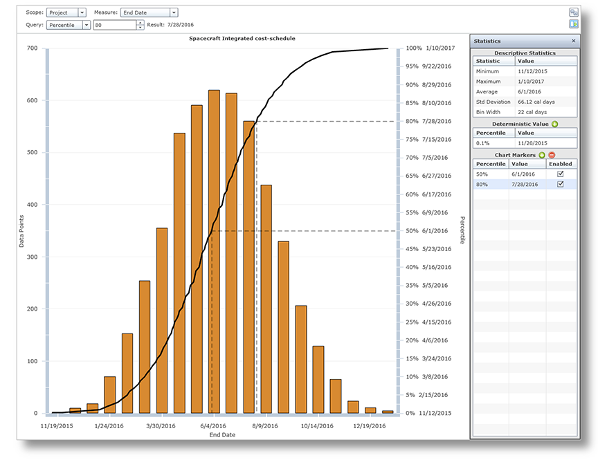
Figure 2 presents another output, from a resource-loaded schedule, illustrating an integrated cost-schedule risk analysis. The upward slant of the time-cost scatter diagram represents the fact that time and cost of a project are related because longer schedule durations for labor-type resources generally generate higher costs (depending to some extent on the type of contract). Each dot represents the finish date and total cost of the project with a possible set of uncertainty and risks. The cross‑hairs of the scatter diagram shows one possible combination of finish date and cost that would produce about a 70 percent probability of success in both time and cost parameters.
Figure 2
Scatter Diagram Illustrating Finish Date and Cost Results
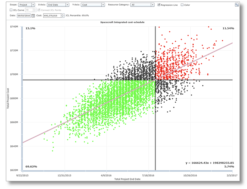
Notice that for each possible finish date (X-axis) there are many possible costs (Y-axis). An organization might choose to schedule and price to these dates for a 70 percent chance of joint cost and schedule success.1
3. KEY ELEMENTS IN QUANTITATIVE RISK ANALYSIS
The key elements of a quantitative schedule risk analysis are discussed below.
3.1 THE SUMMARY PROJECT SCHEDULE
The platform for cost schedule integration quantitative risk analysis is the project schedule with costs loaded as summary resources. Since most traditional cost estimates are developed in a spreadsheet, a risk analysis of the project’s cost estimate is often conducted using a software package that simulates a spreadsheet cost model.2 These analyses are often incomplete because it is difficult to represent the schedule risk’s impact on cost in spreadsheet models.
Integrated cost-schedule risk analyses perform Monte Carlo simulations on a resource-loaded project schedule (i.e., logically-linked, comprehensive, Level 2 or Level 3 schedule) so that both schedule risk and cost risk can be analyzed simultaneously in the simulations. Software that is able to simulate schedules developed in the organization’s preferred scheduling package must be used.3
An integrated cost-schedule risk analysis involves a good-quality schedule with resources representing the cost estimate (without contingency) attached to the activities they support. Generally, this schedule is a strategic one that differs from the most detailed schedules used to run the project on a daily basis. An integrated master schedule at Level 2 or better Level 3 can be developed, by the owner’s own schedulers and estimators. It is purposely built for cost schedule integration and consistency with the contractors’ schedules. The summary schedule has fewer (perhaps 500 to 2,000) activities than detailed schedules intended for daily project management. It is developed from the top down to a level where the important interconnections between project areas are represented in logic and where the risks can be appropriately assigned to activities and costs. The schedule should have identifiable paths with calculated total float that is representative of project flexibility in different project areas.
It is not recommended to develop this summary schedule by combining and linking different contractors’ schedules. Contractors’ schedules are generally inconsistent with each other and may not obey scheduling best practices, so they need to be debugged before using. The Level 2 or Level 3 summary schedule should be consistent with the contactor schedules because the project is following the contractors’ plans. The summary schedule will show all of the work, be consistent with best practices, and show the key paths with realistic total float. The schedule needs to be detailed enough to both represent interconnectedness between project areas and also to place risks where they apply.
There are many different catalogues of project scheduling best practices. One of these from the United States Government Accountability Office (GAO) shows ten components of best practices that the Level 3 Integrated Master Schedule must exhibit to be a dynamic model of the project plan and viable platform for Monte Carlo simulation.4 Table 1 below lists the ten best practices:
Table 1
Summary of the United States Government Accountability Office
Scheduling Best Practices
- Capturing all activities in an Integrated Master Schedule (IMS) at a level of detail that is appropriate for its intended use
- Sequencing all activities with logic and duration, avoiding constraints, open ends, and lags
- Assigning resources to all activities for duration estimation and resource management
- Establishing the duration of all activities based on work, resources, productivity, and other factors
- Integrating schedule activities horizontally (see Best Practice #2) and vertically, including all summary representations of the schedule at a point in time
- Establishing the critical path for all activities that reasonably represent the activities crucial to finishing the project
- Identifying float between activities that reasonably represents schedule flexibility
- Conducting a schedule risk analysis using schedule risk best practices
- Updating (statusing) the schedule on a regular basis
- Maintaining a baseline schedule
Notice that the GAO includes conducting a project schedule risk analysis (Best Practice 8) as a part of scheduling. In recognition of the fact that the deterministic schedule completion date is only correct if the activity durations are known with certainty and everything goes according to plan, risk analysis is needed to achieve the goal of estimating when the project will really finish by taking risks into account.
3.2 UNCERTAINTY
An element of risk that may affect the cost and/or duration of a project is uncertainty. Uncertainty includes: inherent variability, estimating error, estimating bias, and unidentified risks. Uncertainty impacts are applied directly to the activity durations and costs generally as multiplicative ranges. Then, in a Monte Carlo simulation, the software pulls at random an impact multiplier from a distribution, often a triangular distribution, for each iteration of the simulation. That impact value, say 107%, then is used to multiply the durations of the activities the risk affects in the model to get the simulation value, which is, therefore, 7 percent longer than the scheduled duration for that iteration.
- Inherent variability comes from people and organizations not being able to perform tasks reliably in accordance to plan. Uncertainty is always present, so it has a probability of 100%. It often has an opportunity and a threat tail such as ‑5% and +5% and usually includes the estimate of duration or cost. This is similar to “common cause variation” described by Walter A. Shewhart and discussed by W. Edwards Deming.5
- Estimating error represents the confidence in the estimates of activity duration or cost element being as estimated. The uncertainty ranges are often specified as a 3-point estimate with low, most likely and high values expressed in multiplicative terms. Adding estimating error to inherent variability would widen the uncertainty range, e.g., to -10% to +10%.
- Estimating bias is often due to inherent optimism, usually to show the project completing earlier or with less cost than would be realistic. Hence, the optimistic tail of the distribution may not have as much probability as the pessimistic tail. Also, the most likely value may not be the value in the schedule or estimate. Hence, a fairly typical uncertainty range would be, in triangular form 95%, 105%, and 115%. The values imply that a realistic duration or cost is believed to be most likely 5% higher than in the model.
- Unidentified risks may occur later in the project and cannot be managed proactively because they are unknown. These downstream uncertainties are addressed by allocating to them a wider level of uncertainty than that assigned in the early years of the project. In this way the generally higher level of uncertainty in the later years of the project can be included in the risk analysis leading to the size of the contingency reserve.
Uncertainty is generally viewed as irreducible, so it forms the minimum contingency needed to provide for project schedule and confidence. Finish dates and costs resulting from uncertainty generally provide the very best result (shortest schedule, lowest cost) that the project may take even with aggressive mitigation of discrete risks.
Some types of activities have more inherent uncertainty than others. It may be more difficult to make estimates of duration and cost for testing than for design. Whereas, the uncertainty of fabrication duration or cost may be somewhere in the middle range relative to design and testing. Therefore, some categories of activities may have wider uncertainty ranges than others. These activity-type uncertainty bands are sometimes termed reference ranges.
Finally, individuals are often likely to underestimate the duration ranges even in intense and confidential risk interviews. The well-known anchoring and adjusting bias is often the cause of reported uncertainty ranges that are too narrow.6 A wider range could be used to counteract this tendency, and the “trigen” function is available to produce a wider spread of impact uncertainty than is recorded in the data collection.
3.3 DISCRETE RISKS – RISK DRIVER METHOD
Discrete Risk Events are often identified and quantified in the Risk Register. However, the Risk Register is usually incomplete, so risks that are not yet identified in the Risk Register may be discovered when interviewing for risk data to use in the quantitative schedule risk analysis. The risks are quantified by their probability and impact, if they happen, on activity durations or cost elements and correlated to those activities and costs that they affect. The discrete risks are often thought of as being reducible by mitigation (for threats) or expansible by enhancement (for opportunities). Discrete risks are similar to the concept of special cause variation.7
Discrete risks are often thought of as being reducible, to some extent, to provide an earlier date or lower cost than results from all risks before mitigation. Discrete risks are generally not completely mitigatable. The Risk Driver Method8 concepts include:
- The risk probability determines the fraction of the Monte Carlo iterations in which the risk appears. These iterations are chosen at random during simulation.
- The risk impact range is related to the duration of activities or size of cost line items to which they are assigned. Hence, the impact range is not the same concept as that used for qualitative risk analysis, which is impact on the final date or total cost.
- The discrete risk is assigned to identified activities or cost elements the risk affects if it occurs. A risk can affect many activities or cost elements. Activities or cost elements can be affected by more than one, sometimes many, discrete risks.
- Discrete risks can be represented by adding a risk to a cost element or schedule activity or by specifying a multiplicative factor to apply to the estimated cost (Risk Register method) or activity duration (Risk Driver method used in this article).
Possible discontinuous events such as failing a qualifying test can have consequences beyond adding duration to existing activities or cost to an existing budget element. Failing a test (or other discontinuous events) may require adding activities to the schedule and cost line items that represent recovery from the event. Such activities often include a task for root cause analysis of the incident, planning the recovery, executing the recovery and then re-testing the article that failed. These activities and cost elements are almost certain not to be in the schedule or cost estimate because those artifacts are usually based upon success, not failure.
3.4 GOOD QUALITY RISK DATA – COLLECTION METHODS
Good quality risk data are both important to the quality of the risk analysis and also difficult to collect. Mostly, we do not have data about individual risks. Historical performance data reflects many influences acting simultaneously. It is impossible to separate uncertainty from the discrete risk events using historical data and to separate the impact of one risk event from another. As a result, risk data are usually gathered by relying on the expert judgment of experienced people with knowledge of the project or similar projects.
People at all levels, from team members to corporate management, have different perspectives and can contribute insights from their own experience. Gathering data from Subject Matter Experts (SMEs) can take several forms, from carefully planned voting experiments, group risk workshops, or individual interviews. Each of these has its place, but our experience is that individual risk interviews conducted in confidence have crucial benefits by enhancing the quality of the risk data used in the analysis. Using the best quality risk data available is key to the success and usefulness of the results of a risk analysis.
One crucial component of the risk data is the identification of the main risks to project schedule and cost success. These data are often thought to be included in the Risk Register. Experience has shown that the Risk Registers are incomplete because some risks, often the most important risks, are left out. The evidence for this conclusion is that the list of risks is usually enhanced using confidential interview techniques, because SMEs introduce important risks during the interviews. One possible reason that the Risk Register does not contain these important risks is that risk data are often collected in risk workshops where people are reluctant to speak of some important, unpopular, or potentially very damaging risks for fear of being criticized by others in the room.
The risk interviews are conducted one-on-one with the facilitator and a single project team member, manager, or contractor interviewee. Confidentiality is pledged to the interviewee in the sense that nothing will be revealed outside of the interview room that identifies what any specific interviewer said, such as the introduction of new risks or the probability and impact offered for any of the risks. The interviewees are listed alphabetically so the reader of the report can see who was interviewed but not what any specific interviewee said. We have often had to refuse the request of management to reveal the information provided by individuals.
In this one-on-one discussion about project risk, an individual may experience the most intense discussion about risk experienced to date, being in a room with someone who is focused on his specific answers and in fact encouraging him to discuss those risks in the most concentrated way. Some risks that were “unknown unknowns” before the interview are discussed for the first time and corroborated (or not) by subsequent interviewees.
These interviews, which take on average about two hours each, also uncover risks that are unpopular to discuss in an open setting. In confidential interviews, some of the “unknown knowns” can be discussed. Psychoanalytic philosopher Slavoj Zizek defines the “unknown known” as that risk which we intentionally refuse to acknowledge that we know. German sociologists Daase and Kessler agree with a basic point of former U.S. Secretary of Defense Donald Rumsfeld in stating that the cognitive frame of mind for political practice may be determined by the relationship between what we know, what we do not know, and what we cannot know. In their opinion, Rumsfeld left out “what we do not like to know.”9
3.5 MONTE CARLO SIMULATION METHODS – GOOD QUALITY SIMULATION SOFTWARE
Monte Carlo simulation of a risk-loaded schedule is performed using a professional schedule risk simulation package. We have often chosen Polaris® which is a modern schedule risk analysis software product developed by Booz Allen Hamilton, but other packages such as Oracle Primavera Risk Analysis® can perform the same tasks. Polaris® was developed at the request and with initial funding by NASA, which has established the Joint Confidence Level approach to budgeting and scheduling for many of their projects. The Joint Confidence Level is defined as follows:
For implementation of each major program segment, all space flight and information technology programs are to be baselined or rebaselined and budgeted in accordance with the following:
- There is a 70 percent probability (or a different probability that is approved by the decision authority) of achieving the stated life cycle cost and launch schedule.
- Projects are to be baselined or rebaselined and budgeted at confidence level consistent with the program’s confidence level10
3.6 RISK-SUPPORTIVE ORGANIZATIONAL CULTURE
For a risk analysis to be successful, the organization must be committed to conducting an independent, unbiased, and realistic analysis of project risks and to utilize its output, for example, by applying sufficient resources to achieve realistic cost and schedule objectives, or by prioritizing the risk events to be mitigated in order to improve the prospects of the project. This culture starts at the top of the organization but involves everyone participating in the project and others with staff responsibility. Without supportive management, the risk analysis may be hindered or ignored and will not be used to its fullest potential (e.g., by not executing the recommended mitigation actions). Risk analyses are less successful if they are only being performed to “check a box” on a list or because procedures require the analysis. Some organizations even ignore the presence of project risk entirely. Risk aware organizations, however, can and do benefit from conducting risk analyses.
3.7 CASE STUDY ILLUSTRATING THE STEPS OF A QUANTITATIVE RISK ANALYSIS
The key steps involved in an integrated cost-schedule risk analysis are illustrated in the following case study of an integrated cost-schedule risk analysis for an offshore natural gas production platform construction and installation project.11
3.7.1 The Resource Loaded Project Schedule
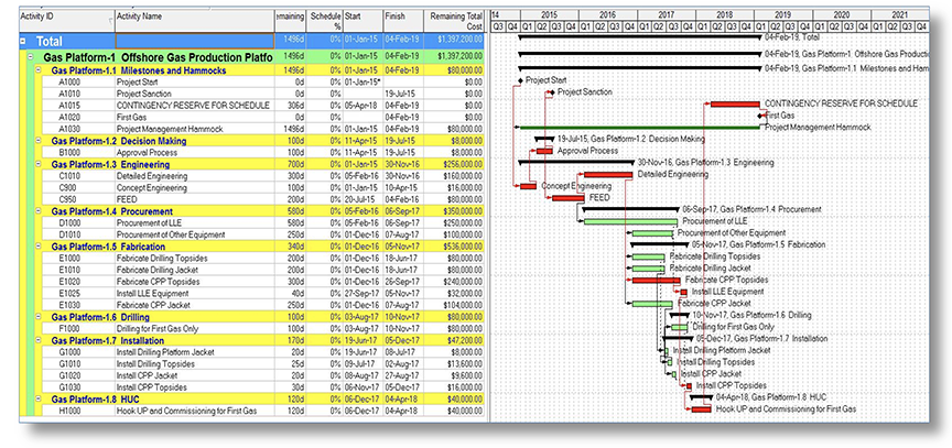
The initial step of the risk analysis involves the development of a resource-loaded project schedule, as shown in Figure 3 below:
Figure 3
Simple Offshore Production Platform Schedule in Primavera® P6
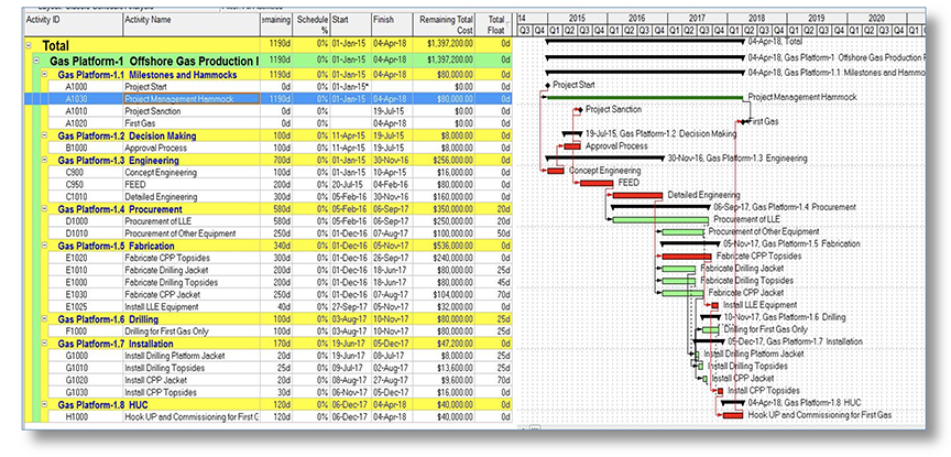
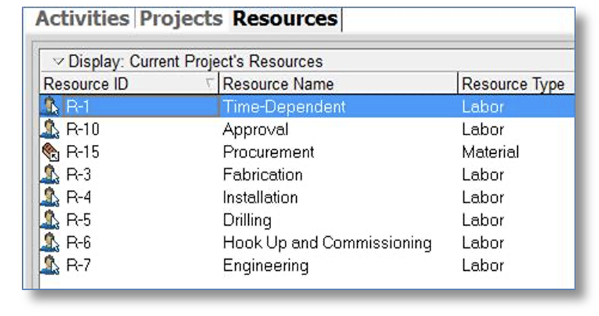
This is a project starting January 1, 2015 and is scheduled to be completed on April 4, 2018 at a cost of $1.397 billion. This cost is expressed without any added contingency because the cost contingency is re-estimated during Monte Carlo simulation while it estimates, perhaps for the first time, a schedule contingency. Resources, used in the analysis, include mostly labor but also equipment in the procurement activities. In this case study, the resources are specified at a summary level as shown in Figure 4 below:
Figure 4
Summary Resources Applied to Activities
3.7.2 Importing the Schedule to Polaris®
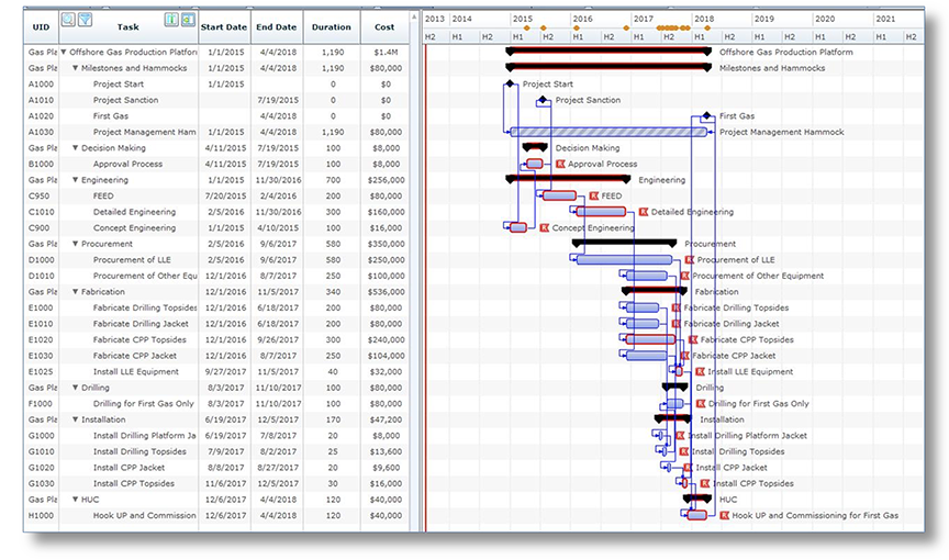
The project schedule is imported from the Primavera® P6 xer file to Polaris® as shown in Figure 5 below:
Figure 5
The Offshore Gas Platform Project Schedule Imported to Polaris®
3.7.3 Applying Uncertainty to Different Types of Activities
The schedule risk analysis starts with uncertainty reference ranges specified to reflect the inherent uncertainty, estimating error, and estimating bias. In the case study, these reference ranges are different for Decision Making, Engineering, Procurement, Fabrication, Drilling, Installation, and Hook-up and Commissioning (HUC). The uncertainty ranges are collected during the interviews. As shown in Figure 6 below, the Trigen function is used to offset the narrow ranges found during the interviews because of the common anchoring and adjusting bias. In this case, the 3‑point estimate is configured to describe 80 percent of the distribution with 10 percent above the high range and 10 percent below the low range.
Figure 6
Assigning Different Uncertainty Ranges to Different Types of Activities

Notice that the uncertainty exhibits fairly narrow ranges and does not represent the impact of discrete risks on the activity durations. The uncertainty ranges are applied to the activities in the named categories by a Trigen distribution from which the computer program pulls at random a multiplicative factor that is applied to the schedule duration. The simulation exercise uses 5,000 iterations because the software is very fast; however, 3,000 iterations would generally be enough to achieve a stable date and cost at the 80th percentile level.
Uncertainty ranges could be wider for work that is being planned and estimated further out into the future. This is because it is harder to estimate durations or costs several years into the future, because the work has not been contracted yet and may not actually be detailed with any specificity. Also, there will be unknown unknowns, namely risks in the future that cannot be identified today but should be provided for with wider uncertainty ranges in the later stages of project execution. A correction factor analysis for downstream uncertainty has not been performed for this case study.
If the uncertainty values applied directly to the durations are not correlated, there will be a good deal of cancelling out as the uncertainty is calculated along the schedule paths and the overall range will be less than specified during the interviews. If an interviewee stated that the duration uncertainty for the project is 90%, 105%, and 120% for the Fabrication activities, applying those ranges to the individual Fabrication activities without correlation will result in a total Fabrication range that is more narrow than the interviewee wanted. Hence, to be faithful to the ranges specified during the interviews, the uncertainties have to be correlated 100 percent. That way, the uncertainty range for the phase or project will approximate the ranges derived from the interviews.
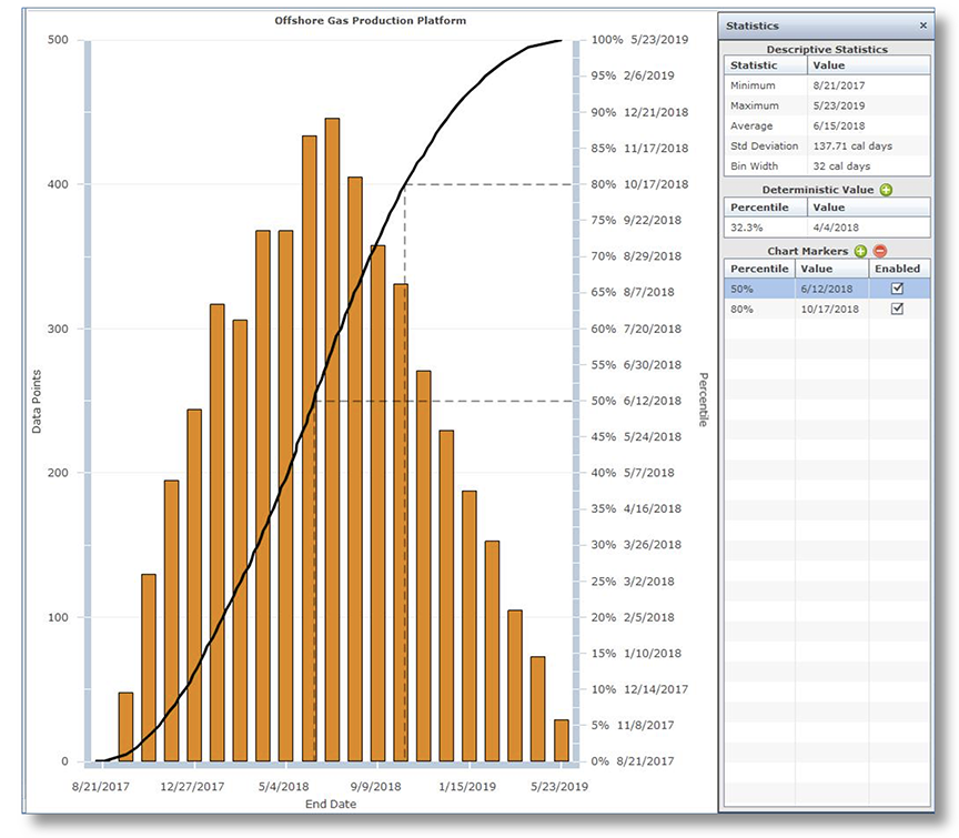
Results from this operation are shown in Figure 7 below. Notice that the P-80 date is now October 17, 2018 or over 6.4 months from the scheduled date of April 4, 2018. However, because correlation between uncertain durations also results in shorter low durations as well as longer high durations, the possibility of finishing on time is 32 percent.
Figure 7
Schedule Risk Results with Uncertainty and 100 Percent Correlation
At this point, the cost risk represents only the effect of duration uncertainty on time-dependent (e.g., direct labor under reimbursable contracts, indirect or level-of-effort labor, construction supervision, and rented equipment) resources. That means that, if the duration on activities with time-dependent resources is longer than scheduled, the cost will be more than estimated. Also, the indirect costs represented in this schedule by the Project Management Hammock activity will cost more as the project generally takes longer.
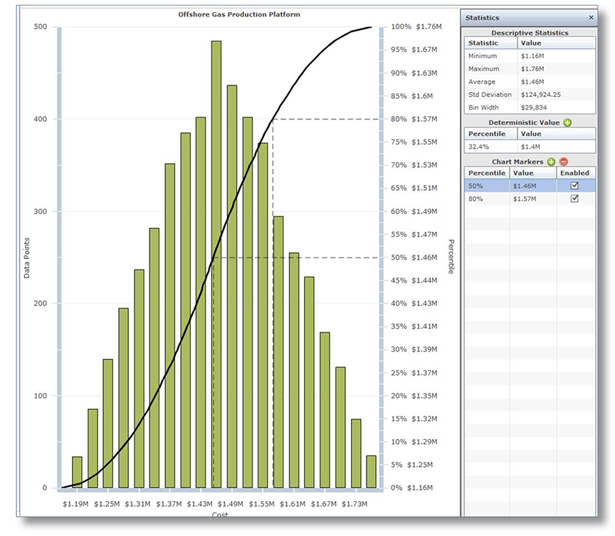
The cost risk results are shown in Figure 8 below. The P-80 cost has increased to $1.57 billion from $1.4 billion with just uncertainty on cost. The increase of $170 million illustrates the importance of integrating the cost risk and the schedule risk.
Figure 8
Cost Risk Results with Uncertainty Driving Time-Dependent Resources’ Costs
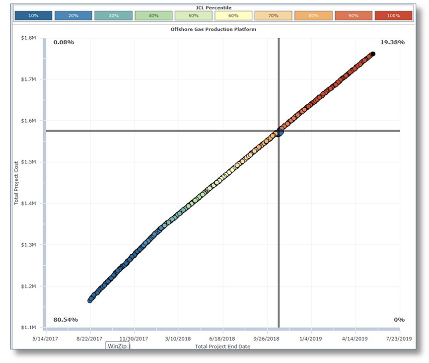
In the scatter diagram shown in Figure 9 below, the finish date and total project cost are correlated 100 percent, illustrating that the schedule duration is the only factor driving cost.
Figure 9
Correlation of Finish Date and Total Cost with
Only Schedule Uncertainty Driving Cost
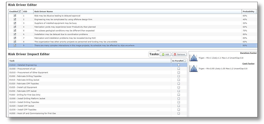
3.7.4 Creating Risk Drivers with Probability, Impact Ranges and Assigning Them to Activities
The next risk modeling step is to identify, calibrate, and assign discrete Risk Drivers to the activities. In this case study, there are nine risks, some of which are assigned to specific categories and some of which are assigned across categories. The latter type of risk is illustrated by Risk 9, “This is by far the largest megaproject conducted by this company…,” which is assigned across the board. The assignment of Risk 9 with its probability and assigned impact ranges is shown in Figure 10 below.
Figure 10
Creating and Assigning Risk Drivers to Activities
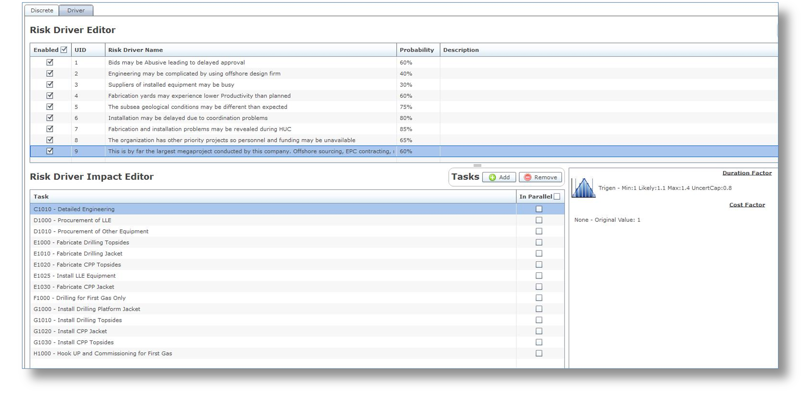
When a Risk Driver is assigned to multiple activities, the durations for those activities become correlated because: 1) if the risk occurs, it occurs for all activities to which it is assigned, and 2) the multiplicative factor chosen for that iteration is applied to all of those activities. As a result, the activities become 100% correlated. If different risks are also assigned to some activities but not all, the correlation between activity durations is reduced. In this way, the Risk Driver method models how correlation occurs so SMEs do not have to guess at the correlation matrix.12
In this case study example, adding Risk Drivers increases schedule and cost risk results at the P‑80 level:
- The P-80 finish date is delayed until August 30, 2019, about 10½ months beyond the October 17, 2018 date with correlated uncertainty only.
- The P-80 cost is $1.9 billion, or $330 million above the $1.57 billion result from correlated uncertainty only.
The scatter diagram is shown in Figure 11 below. The correlation between cost and schedule is still strong at 96 percent, because cost is still being driven only by variability of durations.
Figure 11
Scatter Diagram from Adding Risk Drivers to the Schedule Activities
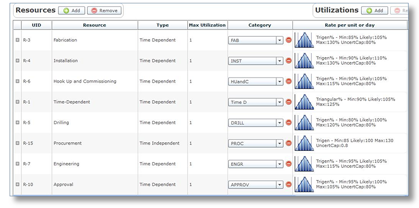
3.7.5 Uncertainty in the Burn Rate and Total Cost
The last consideration in this case study is whether there are uncertainties in the daily “burn rate” of the time dependent activities and in the time-independent resources total cost which would cause cost variations independent of schedule. These cost factors can be entered as the implication of Risk Drivers. Uncertainty applied to different resources is shown in Figure 12 below for this example:
Figure 12
Adding Uncertainty to the Burn Rate for Time-Dependent Resources
Adding uncertainty to the time-dependent burn rate increases the P-80 cost to $2.05 billion from $1.9 billion as shown in Figure 13 below. The P-80 schedule results remain at August 30, 2019. The correlation between the finish date and total cost is reduced to 87 percent.
Figure 13
Effect of Schedule Risk and Burn Rate Uncertainty on Total Cost

Typical project cost risk analysis identifies risks that are specific to costs. These cost risks are represented by Risk Drivers that are given cost risk impacts. When these risks occur, they will vary the burn rate on time-dependent resources and the total cost on time-independent (raw materials, installed equipment) resources. Figure 14 below presents an example of cost Risk Drivers added into the risk analysis model.
Figure 14
Adding Cost Risk Drivers
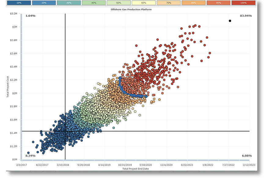
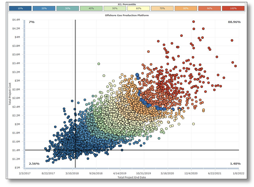
With the added cost Risk Drivers, the total cost at the P-80 level increases to $2.34 billion, up from $2.05 billion, with schedule uncertainty and Risk Drivers and uncertainty on resources. The cost and schedule correlation is 76 percent, reduced from 87 percent without the cost Risk Drivers, as shown in Figure 15 below:
Figure 15
Cost and Finish Date Scatter Plot after Adding Cost Risk Drivers
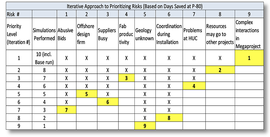
3.7.6 Prioritizing the Risk Drivers
The risks can be prioritized for schedule and/or cost based on the following approach, described for schedule:13
- Run the simulation with uncertainty and all risks. Record the P-80 finish date.
- Run the simulation nine times, each time disabling one of the risks. Record the P-80 date for each run.
- Select the risk that results in the earliest P-80 date. That is the highest-priority risk to mitigate.
- Keeping that risk disabled, perform eight simulations, disabling each of the eight remaining risks one at a time, recording the P-80 date and determining the second most important risk by the earliest such date achieved.
- Repeat this process for each Risk Driver, prioritizing the risks as if they could be completely mitigated, which is used in this process but is unrealistic.
Figure 16 below presents how these simulations occur for the case study and the priority order that each risk has based on this method. It also indicates that 46 simulations are needed to prioritize the nine risks used in this example.
Figure 16
Prioritizing the Risk Drivers for Mitigation
The results of the risk prioritization for schedule are shown in Figures 17 below. The process can be optimized for risk prioritization to cost as well, or to any milestone or activity if needed by a team lead.
Figure 17
Risks Prioritized to Schedule at the P-80 Level of Confidence (Tornado Chart)
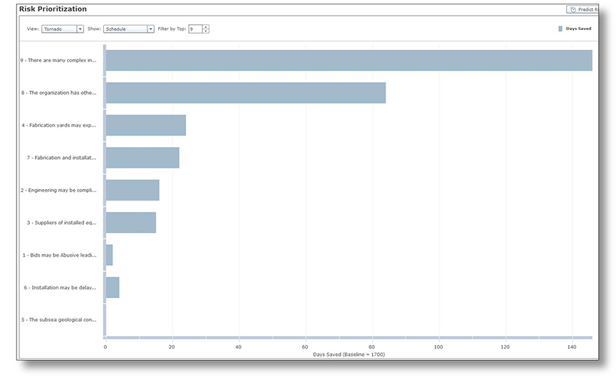
Table 2 below presents the risks prioritized to schedule at the P-80 level of confidence.
Table 2
Risks Prioritized to Schedule at the P-80 Level of Confidence
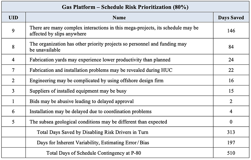
The prioritization of risks is calibrated in “days saved” at the P-80 level of confidence as the risks are disabled in priority order. Management can use these values in benefit-cost calculations of mitigation actions more conveniently than the results from more traditional tornado charts that express their results as correlation coefficients between activities, risks, and total project finish dates.
Often the “days saved” measure does not reduce monotonically down the table of prioritized risks. Inversions may occur because the days saved includes the effect of the project schedule’s logical structure. If one risk is mitigated it may uncover an important risk on a parallel path that has a larger days saved, but only if the higher-priority risk is mitigated. Until the higher-priority risks are address with mitigation, spending time and money mitigating lesser-priority risks will not have much effect. The risks should be addressed in priority order, which is why prioritization is crucial for effective risk mitigation.
If the risks were completely mitigated, about 313 total (calendar) days could be saved out of a schedule contingency of 510 days including uncertainty. A savings of 313 total days is considered an unrealistic outcome because most risks cannot be completely mitigated.
3.7.7 Risk Mitigation Workshops
The risk mitigation exercise should be done in a workshop setting rather than in interviews because many people have to contribute ideas and commit to the mitigations. However, these workshops are not places to argue about the risk analysis results. The results come from the schedule model, risk data from many interviews, and the Monte Carlo simulation method that is over 60 years old. Risk mitigation workshops and analyses may be structured as follows:
- The risk mitigation workshop participants typically include the Project Manager, Deputy Project Manager, team leads, and others involved in mitigation of risk.
- Given the prioritized list of risks for a project that may overrun cost and schedule targets, the workshop team can develop risk mitigation actions. The workshop participants estimate the improvement in the probability and impact parameters that are expected to result from the various mitigations planned for each identified risk (uncertainty cannot be mitigated in concept). Risk owners and a rough estimate of the cost of the mitigation action are recorded.
- A post-mitigation resource-loaded schedule is created with the probability and impact parameters that resulted from the risk mitigation workshop. Each risk mitigation action accepted is modeled. Comparing the results of the pre-mitigation and post-mitigation simulations will determine how much benefit is expected from the mitigations.
- For the mitigation actions to “count” against the project risk, the project and the organization’s management must commit to them. This commitment is evidenced by inclusion of mitigation actions in the post-mitigation budget and schedule, and assignment of people to monitor the risks and their mitigations. These risks should be added to the Risk Register as well, so they are reviewed frequently.
- The final report includes post-risk mitigation results and the overall project cost and schedule risk if those risk mitigation actions are taken to mitigate the risks. Note that the original cost and schedule target will generally not be met because that would require complete mitigation of the risks that caused the estimate of overrun in the risk analysis itself.
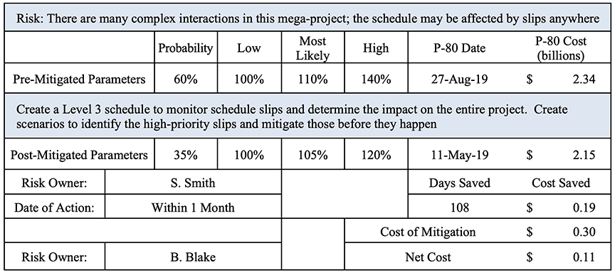
Table 3 below presents an example of a typical risk mitigation resulting from a Risk Mitigation Workshop:
Table 3
Typical Risk Mitigation Derived from a Risk Mitigation Workshop
3.7.8 Add Post-Mitigation Time Contingency to the Schedule
It is becoming more common to add a contingency reserve to the end of the project schedule before final turnover (First Gas in this case study) based on the post-mitigation results from the risk analysis. Figure 18 below shows an acceptable way to add the contingency just before the finish date.14
Figure 18
Adding a Contingency Reserve of Time to the Project Schedule
4. SUMMARY CONCLUSIONS
Project schedules and costs are subject to uncertainty and risks. The validity of the schedule’s finish date and the total cost estimate should be examined by a risk analysis that addresses both uncertainty and risk for both schedule and cost. The method of approach is to:
- Create a summary schedule at Level 2 or Level 3 that is integrated, logically-linked, and complies with scheduling best practices. The budget or cost estimate is incorporated into the schedule with summary time-dependent and time-independent resources assigned to activities.
- Gather data about uncertainty and risk. Experience has shown that individual confidential interviews of subject matter experts in the project teams and management, contractors, and other knowledgeable personnel in the organization, can uncover risks that are either new or unpopular to discuss in risk workshops.
- Use a modern Monte Carlo schedule risk analysis software package to model both uncertainties to activity durations and to time-dependent resources’ burn rates or time-dependent resources’ total material costs.
- Prioritize the Risk Drivers to schedule and to cost (only schedule was illustrated above).
- Prepare a pre-mitigated risk results presentation.
- Conduct a risk mitigation workshop using the prioritized risks contained in the pre-mitigation presentation as a guide to the most important risks.
- Gain organizational commitment to those mitigation actions to be adopted, scheduled, budgeted, staffed, and monitored.
- Prepare a post-mitigation model and simulate it.
- Prepare a post-mitigation report.
Experience has shown that project management and sponsoring organizations gain insight into their projects, improve the possibility of project success, and experience fewer costly surprises if they conduct schedule risk analyses periodically throughout project planning, engineering, procurement, execution, and commissioning.
About the Authors
David T. Hulett, Ph.D., FAACE, is a Cost & Schedule Risk Analysis Partner affiliated with Long International. He has conducted many risk analyses, focusing on quantifying the risks and their implications for project cost and schedule, and many schedule assessments. Dr. Hulett is a Principal with Hulett & Associates, LLC (H&A), and has focused for nearly 30 years on quantitative schedule risk analysis, integrated cost-schedule risk analysis, and project scheduling best practices. H&A clients are in oil and gas, aerospace, construction, pharmaceuticals, and transportation. They are located in the U.S., Canada, South America, Southeast Asia, Europe and the Middle East. H&A has pioneered the Risk Drivers approach to schedule risk and integrated cost and schedule risk analysis and he has recommended adopting this method for new and emerging Monte Carlo software to serve the needs of his high-end risk analysis customers. Dr. Hulett has experience in applying Risk Drivers to large multi-year projects leading to proactive risk mitigation planning for better project results. From these analyses, the client learns: the probability of achieving the cost and schedule with the existing project plan, the amount of time and cost contingency required to achieve a desired level of certainty, which priority risks drove the analysis results, and which risk mitigation actions address the risks. Dr. Hulett is based in Los Angeles, California and can be contacted at dhulett@long-intl.com and (310) 476-7699.
Andrew Avalon, P.E., PSP, is Chairman and CEO of Long International, Inc. and has over 35years of engineering, construction management, project management, and claims consulting experience. He is an expert in the preparation and evaluation of construction claims, insurance claims, schedule delay analysis, entitlement analysis, arbitration/litigation support and dispute resolution. He has prepared more than thirty CPM schedule delay analyses, written expert witness reports, and testified in deposition, mediation, and arbitration. In addition, Mr. Avalon has published numerous articles on the subjects of CPM schedule delay analysis and entitlement issues affecting construction claims and is a contributor to AACE® International’s Recommended Practice No. 29R-03 for Forensic Schedule Analysis. Mr. Avalon has U.S. and international experience in petrochemical, oil refining, commercial, educational, medical, correctional facility, transportation, dam, wharf, wastewater treatment, and coal and nuclear power projects. Mr. Avalon earned both a B.S., Mechanical Engineering, and a B.A., English, from Stanford University. Mr. Avalon is based in Orlando, Florida and can be contacted at aavalon@long-intl.com and (407) 445-0825.
1 NASA has adopted this 70 percent target as a way to schedule and price their projects and has gained recognition for better project management, mainly because of the increased realism of its cost and schedule forecasts.
2 Two commonly used packages are @RISK® from Palisade Corporation and Crystal Ball® from Oracle.
3 There are several schedule simulation packages available. Two of the most capable schedule simulation packages are Polaris® from Booz Allen Hamilton and Primavera Risk Analysis® from Oracle.
4 The GAO Schedule Assessment Guide: Best Practices for Project Schedules, published as an exposure draft for comment in 2012, can be found at http://www.gao.gov/products/GAO-12-120G. The publication of the final Guide is planned for 2015.
5 Lean Six Sigma Dictionary, “Common Cause Variation,” http://www.isixsigma.com/dictionary/common-cause-variation.
6 Amos Tversky and Daniel Kahneman, “Judgment under Uncertainty: Heuristics and Biases,” Science, September 27, 1974.
7 Lean Six Sigma Dictionary, “Variation (Special Cause),” http://www.isixsigma.com/dictionary/variation-special-cause.
8 The Risk Driver Method is described in David Hulett, Practical Schedule Risk Analysis (2009, Gower Publishers), Chapter 8.
9 Wikipedia, “There are known knowns,” http://en.wikipedia.org/wiki/There_are_known_knowns.
10 NASA HQ – Office of Program Analysis and Evaluation Cost Analysis Division, “Joint Confidence Level (JCL) FAQ,” http://www.nasa.gov/pdf/394931main_JCL_FAQ_10_12_09.pdf.
11 These key steps are also described in David Hulett, Principal Author, “Recommended Practice 57R-09, Integrated Cost and Schedule Risk Analysis using Monte Carlo Simulation of a CPM Model,” AACEI, 2011.
12 This correlation of activity durations due to mutually assigned risks is different from the 100 percent correlation between activities assigned with uncertainty. These two assumptions can exist simultaneously.
13 Polaris® appears to be the only schedule-cost simulation program that has automated this method of risk prioritization. Other software solutions use traditional tornado diagrams that mainly report on correlation between activities and finish date, or between risks and finish dates, so this prioritization must be done manually.
14 It is not prudent to try to spread this contingency time to the activities or key milestones, because schedule contingency (e.g., at the P‑80 level of confidence) was determined by an overall risk analysis with risks on most activities and paths, culminating only at the finish milestone.
Copyright © Long International, Inc.
ADDITIONAL RESOURCES

Articles
Articles by our engineering and construction claims experts cover topics ranging from acceleration to why claims occur.
MORE

Blog
Discover industry insights on construction disputes and claims, project management, risk analysis, and more.
MORE

Publications
We are committed to sharing industry knowledge through publication of our books and presentations.
MORE