
Journey Map to a More Mature Schedule Risk Analysis Process
This article lays out a risk analysis maturity model that allows organizations to determine: (1) where they are today on the scale from “not aware” to “advanced integrated cost-schedule risk analysis” and (2) where they want to be, what is their optimal level of risk analysis maturity.
1. ABSTRACT
Organizations vary in their appreciation of the potential impact of the risks that could affect their achieving time and cost goals while completing the project’s scope. This article lays out a schedule risk analysis maturity model that allows project management to determine: (1) where they are today on the scale from “not aware” to “advanced integrated cost-schedule risk analysis” and (2) where they want to be, what is their optimal level of risk analysis maturity. The levels of maturity are described along with their benefits and properties including tools and outputs that distinguish them from other maturity levels. [For a brief discussion of cost risk maturity, see 11, p. 210.] This article does not mandate that organizations strive to achieve full advanced cost-schedule integration methods and tools (level 5) unless that is desired. Often some projects will require more or less risk analysis maturity depending on size, complexity, type of project or other criteria. This article was first presented as RISK.2890 at the 2018 AACE International Conference & Expo.
2. INTRODUCTION
Advancing the maturity level of an organization’s Schedule Risk Analysis (SRA) process is the responsibility of both the organization’s leadership that instill the risk aware culture and individual employees who implement and participate in it.
2.1 Organizational SRA Maturity
The organization needs to assess its current risk-aware corporate maturity and then set goals to become more risk analysis-mature, if desired. Those actions are key success factors for risk analysis and management maturity. Risk-aware leadership demonstrates needing information about project risk, the “good, bad and ugly” of projects to be more successful in managing all three. The organization’s leadership should demonstrate that it needs the results of the SRA to make decisions. Also, the risk-mature leadership does not tolerate actions or attitudes that punish, impede, bias or prohibit the discussion of potential threats to the program’s finishing date.
2.2 Individual Schedule Risk Analysis Maturity
Risk analysis progression can be described as a graduated set of steps of greater SRA maturity. The journey toward the highest levels of risk analysis maturity requires a risk-oriented awareness, as well as specific risk analysis and supporting skills. It is a multi-attribute process that includes personal attitudes, understanding of more modern and sophisticated methods and where they apply, getting the right training for the maturity level to be achieved, having available and learning the right tools and gaining the practice and experience needed to bring it all together in an integrated process. Some of the tools and capabilities are directly related to schedule risk analysis while others are key capabilities and tools that perform supporting roles such as project scheduling or data gathering by risk workshops or confidential interviews. As well as the risk analysis skills described below, the well-rounded risk-mature individual should master all of the supporting skills that are needed for the current and higher-level maturity. This article does not cover some advanced risk analysis features, such as probabilistic branching or probabilistic calendars. It is focused on the basic differences between maturity levels, the way risk to activity duration (and to cost at maturity level 5) is handled at each level, and the benefits and weaknesses at each level.
2.3 Seeking Risk Analysis Maturity – Where Are You Comfortable?
Not all organizations need to achieve the highest level of risk analysis maturity, though the lowest levels should be soon left behind in favor of methods that follow recognized principles and provide management with actionable information on project risk that will contribute to decision making.
The lowest levels of schedule risk analysis can be implemented without specialized tools and training, although there are software tools that may help the application of, say, qualitative risk analysis (level 2 as indicated in Figure 1).. The highest maturity levels, those involving quantitative risk analysis, require specialized tools that implement Monte Carlo simulation, with training and gaining experience in skills that some organizations do not have at the outset of the risk analysis journey toward higher maturity.
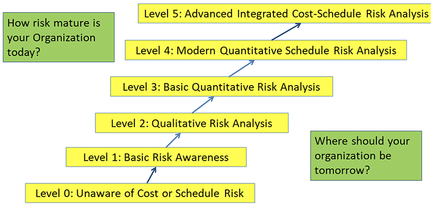
The journey-map shown in Figure 1 will give some organizations a place to be comfortable in practicing risk analysis on projects. They may choose to practice different levels of maturity on different classes (e.g., sizes) of projects. Their choice should also take into consideration the desires of the owner or customer who might need more assurance than the contractor. Every organization, except the most risk mature, will find a description of the next highest aspirational step.
Participating in the organization’s SRA process is the responsibility of most people assigned to the project’s concept, design, execution, commissioning and control. Others that bear the responsibility include those in health-safety-security-environment, regulatory compliance, legal, financial, strategic planning and other areas. Individual employees who implement and participate in the risk analysis and management process may be specifically assigned risk analysis activities, but all can contribute from their experience and observations.
2.4 The Step-Wise Journey of Schedule Risk Analysis Practitioners
The steps in order of increasing risk analysis maturity can be called by various names, but these six describe the path the fully mature SRA professional-practitioner will probably follow:
0 Unaware of Schedule Risk Issues
1 Risk Awareness
2 Qualitative Risk Analysis
3 Basic Quantitative Schedule Risk Analysis (traditional, activity range estimating)
4 Modern Quantitative Schedule Risk Analysis (modern, Risk Drivers Method)
5 Advanced Integrated Cost-Schedule Risk Analysis (using the Joint Confidence Level Method)
Starting with level 2, these are the skills in order of their awareness and tool development for the profession as a whole. Some in the SRA profession have not progressed beyond levels 2 or 3, but the profession has done so.
Contributors to Achieving the Next Level Include:
- Participate in appropriate training in project risk concepts and analysis (concepts familiarity)
- Learn the risk analysis software as needed to participate in the next level (tools proficiency)
- Perform risk analyses mentored by those more “risk mature” (serving apprenticeship)
- Perform risk analyses as leader of the analysis team (displaying capability and leadership)
- Supervise others less “risk mature” (sharing with others)
- Create an organization-wide database of past projects with their characteristics and performance results, normalized to reflect overruns experienced from schedules promoted at the sanction step. The database will have the benefit of providing an “outside view” against which to measure the results from quantitative risk analysis
2.5 Pictorial View of the Risk Analysis Maturity Levels
Each level of risk analysis maturity, except level 5, has a successively more mature level:
Figure 1: Risk Analysis Maturity Levels
3. LEVEL 0: UNAWARE OF COST OR SCHEDULE RISK
The project manager and teams rely on the project scheduling software to provide dates for key milestones and project completion. Nobody questions the duration inputs or the computed project finish date and other results of that exercise. Project management fails to question project assumptions underlying the schedule.
3.1 Distinguishing Features at Level 0
- Individuals rely entirely on the results, specifically the milestone and project finish dates that result from running project scheduling software. They defend those dates.
- Individuals are not alert to any threat to achieving the finish date produced by the schedule.
- They deny and/or refuse to discuss any items that might put the schedule in jeopardy.
- When faced with contrary results from other projects risk-unaware individuals will claim “this project is different” or “it won’t happen on my project.”
- Project management and leaders claim that they “know how to manage” even if their past performance on projects included overruns in the schedule.
3.2 Weaknesses at Level 0
The organization may attempt to rely on and support the schedule software’s result long after it becomes obvious the project is not performing to those dates. Risks are not addressed so they may happen when they could be avoided or their impact on the schedule may be larger than necessary. Surprises and “firefighting” responses after the risk occurs are common at this level of maturity.
4. LEVEL 1: BASIC RISK AWARENESS
This level indicates awareness of project risk as something to consider when reviewing on or reporting using the project scheduling software’s calculated finish date to determine when the project may finish. It represents opening people’s eyes to the benefits of probabilistic thinking about projects without necessarily being able to conduct organized risk analysis or recognizing that there are processes and tools to help them.
4.1 Distinguishing Features at Level 1
This level is characterized by the lack of a systematic way to think about risks. Risk may be discussed frequently and decisions may take account of the risk posed by alternatives, but the influence of risk is not analyzed or universally required before decisions are made. Many organizations perform informal risk management in this way without benefitting from the use of systematic methodologies available today. The success or failure to address risk depends on the intelligence and awareness level of organizational management.
Individuals at this maturity level show awareness about activity duration uncertainty and exhibit willingness to examine assumptions that underlie the schedule. These attitudes imply that the organization is questioning the deterministic scheduling results without necessarily having the tools or systems to examine the role of risks and uncertainty directly.
At this basic level of risk maturity is awareness that the schedule is only correct when the durations are known with certainty and things go according to plan. The organization realizes that “go according to plan” occurs infrequently and that to improve on the deterministic plan requires recognizing and dealing with risks to the activity durations. The risk aware organization may realize that it does not know the finish date just by looking at the results of even the most sophisticated scheduling software tool, but it has no organized structure or tools to help it proceed beyond this awareness.
4.2 Capabilities Required at Level 1
The main tools are awareness at the top of the organization that project schedule cannot be assured. Project team meetings are conducted to discuss the project’s prospects of finishing on time. Any risk management at this level relies exclusively on management’s experience and ad-hoc approaches that are discussed in various project or team meetings.
The ability to think and talk freely and candidly about uncertainty that could affect the schedule durations and the view of whether the schedule is realistic may be found. The organization will probably need to address and enhance the ability to identify and combat barriers to free and open discussion of risks that could affect the schedule.
Individuals could look at the project in light of the results of actual projects with similar outcomes to consider what to expect. This approach has been called the “outside view” following Daniel Kahneman.6, 8
4.3 Benefits/Strengths at Level 1
If a project schedule has been developed, the risk team may recognize whether the activity durations have been biased, usually to produce an earlier finish date, by forces such as management mandates, customer or competitive pressure, etc. If scheduling bias is discovered, the schedule may be re‑baselined.
To achieve this level of schedule risk analysis maturity, individuals need to adopt a way of thinking probabilistically about finish dates that may differ from the deterministic way they were taught or became accustomed to while in their prior experience. This attitude about risk affecting schedule milestone dates may require practice. It will certainly require management’s reinforcement by the organization’s risk culture.
4.4 Weaknesses at Level 1
Since the risks are not addressed in an organized way, some important risks may be overlooked. Even with the risks that have been identified they may not be the root causes of schedule variability. This level lacks an organized way of calculating how individual risks affect the schedule through the probability, impact if it occurs, the activities they affect and the complex logical relationships that cause the risk to affect the risk-critical paths and hence the finish date. While a risk may seem to be important, it may not be the most important, and at level 1 there is no mechanism to prioritize the risks to determine which to address first. At level 1 addressing risks is ad hoc and therefore may be quite inefficient.
5. LEVEL 2: QUALITATIVE RISK ANALYSIS MATURITY
This level of maturity represents examining project risk to schedule (and to other objectives such as cost, quality and scope) using qualitative methods that lead to developing a project risk register.14, 15, 20
5.1 Distinguishing Features at Level 2
Qualitative risk analysis is often viewed as a low-cost and easily-understood but organized method of addressing project risks. Maturity at level 2 may be sufficient for some projects or some organizations. Many organizations manage project risk including risk handling using the risk register that includes scoring risks as high, moderate and low importance to the project objective being examined.
5.2 Capabilities Required at Level 2
Included in this group of capabilities to be reinforced are:
- Ability to identify and name project risks by the sentence structure of “cause (a fact) leads to something that may happen (the risk) that has consequences (the impact).” This structure helps the organization focus on the uncertainty that may happen rather than confuse it with the cause that is a fact or the effect that is the result or symptom of the risk projected on the project.
- Ability to understand a risk’s probability as the concept that a risk will happen to the extent of affecting the project finish date to a greater or lesser degree, in other words, “uncertainty that matters.”
- Ability to estimate within a range the effects of a risk occurring on the project finish date (and other objective such as cost, quality and scope).
- Ability to participate in or even lead a risk workshop to help identify and estimate the probability and impact parameters.
- Qualitative risk functionality leads to the ability to create and maintain a Project Risk Register. Done well, the risk register helps management identify and handle effectively individual risks.
- There are some software tools that support risk register development but standard spreadsheet tools are often used effectively.
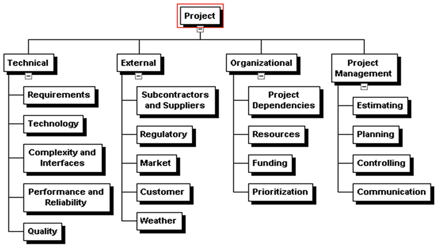
Qualitative risk analysis has benefits of being simple and easily complied with. A useful tool to identify the risks is the Risk Breakdown Structure (RBS), a generalized example, [See 14, 15 for other examples] to be tailored to the specific project before being used in risk identification, is shown in Figure 2. The RBS should help the organization to realize that the causes of risks come from many directions. Risk identification should not only address technical risk but also risk arising from external, organizational and even project management sources.
Figure 2: Typical Risk Breakdown Structure
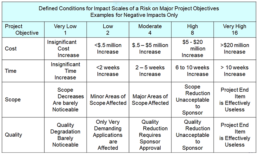
The impact of risks on the total project objective selected must be defined for the qualitative risk exercise by project management. This permits the assessment of risks’ impact to be assessed using compatible measures so the risks’ importance can be assessed relative to each other. An example of the definitions of impact at five levels from very low to very high and for four different objectives is shown in Figure 3. [See 14, 15, 20 for other examples.] These definitions need to be scaled appropriately for the project at hand. These definitions should be tailored to the specific project (e.g., planned overall duration and cost), and the organization’s risk tolerance for a specific project. This figure should be tailored to the project as well as to the organization’s risk tolerance.
Figure 3: Typical Definitions of Impact
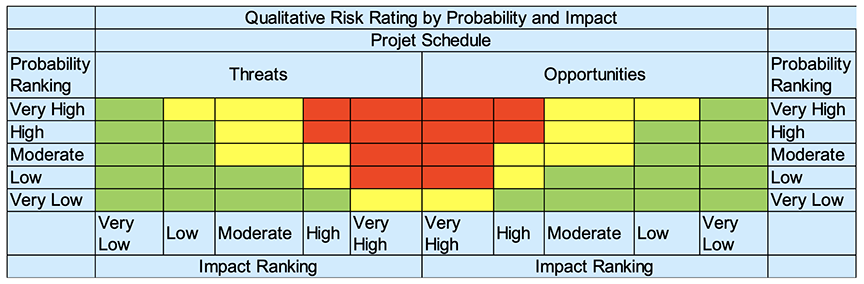
The project manager needs to determine which combinations of probability and impact warrant a “red,” yellow” or “green” condition as shown in Figure 4. The zones of the probability and impact matrix that are designated as low, moderate or high risk needs to be established by management in view of the definitions established and the specifics of the project at hand. Risks should be evaluated separately for their impact on time, cost and quality. Quite frequently projects emphasize either schedule (“schedule driven”) or cost (“cost driven”). Risks may be more important for the project depending on which objective is affected. A simple probability and impact (PxI) matrix for both threats and opportunities is shown in Figure 4. [See 14, 15 for other examples.] The ranges of probability and impact that qualify as red, yellow and green need to be consistent with the probability and impact range definitions such as those in Figure 3. The combinations of probability and impact that show as red in the red-yellow-green scheme are viewed as the most important and serve as the Attention Arrow, coined by David Hillson.18
Figure 4: Classifying Risk by Their Probability and Impact
5.3 Benefits/Strengths at Level 2
Handling risk at maturity level 2 is often enough for many projects. The smaller, shorter-duration, lower-cost projects that do not affect the commitments or reputation of the organization might be handled with the development and maintenance of a risk register.
The risk register can also record the mitigation of risks and their assessed improvement in lowering the probability, reducing the impact, or both. More elaborate risk register approaches will display the timing of the mitigation and a waterfall of planned improvement in the outlook associated with that risk.
5.4 Weaknesses at Level 2
There are limitations to this method of handling project risks:
- It does not provide an estimate of the probability that the scheduled finish date will be overrun or the amount of contingency that should be added to the schedule to provide a desired level of certainty. This is because: (a) each risk is assessed independently and the risks are not analyzed simultaneously as if they may occur, with their probabilities, on the project, and (b) the risks are not analyzed within the framework of the project schedule so the analysis does not account for the structure of the strategic project plan.
- Gauging the impact of a risk on the finish date, which is required for the PxI matrix, implies a basic understanding of which activities within the project schedule are affected by the risk, whether it is on a risk critical path or not, and its effect given that uncertainty and other risks are also potentially at work. In practice, thinking this deeply and in this much detail during the risk data collection phase is hardly ever done in part because it is so difficult. This analysis is particularly difficult without the benefit of the project schedule as a framework for cause-effect analysis.
- Risks are often identified and calibrated in risk workshops. Risk workshops often omit or avoid some of the most important risks that are known but not talked about, called the “unknown knowns.”17 Hence, the risk registers often omit some of the most important but embarrassing risks.
- Some people put numbers 1-to-5 to the probability and impact ranges and then treat these numbers as if they were cardinal values to be multiplied together to determine the red-yellow-green shading of the cells in the PxI matrix. (This is called “semi-quantitative” analysis in some risk management standards.) Handling these probability or impact levels as cardinal numbers that can be added, multiplied, or otherwise numerically compared is a fallacy. In fact, the impact ranges are ordinal so that high impact (4) is higher than low impact (2) but not necessarily twice as bad – just relatively higher. These numbers cannot be added, multiplied, divided or otherwise mathematically manipulated.
6. LEVEL 3: BASIC QUANTITATIVE SCHEDULE RISK ANALYSIS MATURITY
Maturity level 3 recognizes that project schedule success is affected by uncertainty of the estimated durations of the activities in the project schedule and can be analyzed statistically by applying Monte Carlo simulation (MCS) with specialized but available software.
6.1 Distinguishing Features at Level 3
At maturity level 3, possible fluctuations of activity durations from planned is represented by applying, directly to the activity durations individually, probability distributions, typically described with a 3-point estimate of possible days representing minimum (low, optimistic), most likely, and maximum (high, pessimistic) days. The 3-point impact is assessed for the activity durations, often using workshops or interviews of the activity leaders. At this level, the 3-point estimate represents the influence of all risks and uncertainty that would cause the activity’s duration to fluctuate. Probability distributions such as those shown in Figure 5 are used. The schedule model is computed or “iterated” many times using specialized Monte Carlo schedule risk analysis software that imports a critical path method (CPM) schedule from scheduling software. Each iteration of the schedule produces a finish date (and other schedule data) for the project that is consistent with the CPM logic and the activity durations chosen at random for the duration of each uncertain activity for that iteration.
The results are shown by a histogram and cumulative distribution of possible finish dates consistent with the assumptions applied as shown in Figure 6.
6.2 Capabilities Required at Level 3
Skills required at this level of maturity include an ability to understand and assess the quality of the project schedule used in the analysis. Many mature SRA practitioners have become competent in project scheduling including the theory and concepts, as well as learning the scheduling software available of necessity, since many schedules do not comply with best practices. This means becoming familiar with scheduling best practices.7
Activity duration ranges are collected from project participants in interviews or in workshops. Individuals can provide 3-point estimates from their own analyses and experiences on past projects.
Figure 5: Probability Distributions Commonly Used at Maturity Level 3
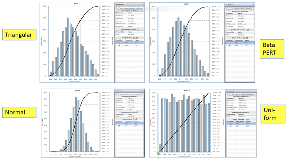
Practitioners at this level of maturity need to understand the fundamentals of probability and of Monte Carlo simulation software at a conceptual and intuitive level. Happily, the mathematics and statistics required are provided by the software.
Most Monte Carlo software built to simulate schedules until the late 1990s uses this method, which applies activity variability distributions directly to activities’ durations without specifying the risks that could cause that variability. This method is still used today by many risk analysts at this maturity level.
6.3 Benefits/Strengths at Level 3
Applying probability distributions directly to the activity durations (or cost line items) has the benefit in that it facilitates Monte Carlo simulations and provides assessments of the project finish date using the project schedule.
The use of the schedule platform avoids some of the weaknesses of level 2 qualitative/risk register analysis because it substitutes the project plan’s logical relationships and the calculations of the results based on that schedule using Monte Carlo simulation software instead of the human brain’s attempt to calibrate the impact of the risk register risk on the project completion date. It also provides a probability distribution of the possible finish date of the project, see Figure 6, that was not available at maturity level 2.
The methods at level 3 use the project schedule that is a comprehensive tool describing the project plan. This platform can handle project risk that affects different paths through the schedule consistent with the logic of the plan that includes parallel paths and merge points. Hence, this method recognizes the important contribution to schedule risk of the merge bias19 that may occur when an activity or milestone has two or more predecessors and the schedule impact of the risk along the shorter path exceeds the free float at that merge point.
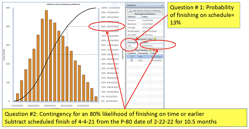
Simulation of the project schedule provides results that are not available from the qualitative risk register methods at level 2. Key information needed to manage the project includes the probability of finishing by the scheduled date and the amount of days contingency required to provide a targeted level of certainty (e.g., the P-80), which are shown by the cumulative distribution. Figure 6 shows the output from a Monte Carlo Simulation and highlights the 80th percentile (P-80) date, as well as the probability of finishing as scheduled.
Figure 6: Typical Schedule Risk Analysis Result
6.4 Weaknesses at Level 3
Most of the weakness at maturity level 3 revolves around the lack of identifying and modeling identified risks because the probability distributions are applied directly to activity durations. These distributions must incorporate the influence of all sources of uncertainty and identifiable risks. These distributions, placed directly on the activity durations rarely, if ever, incorporate the notion that the risks have probability of occurring in addition to impact on durations. Essentially these activity duration distributions represent the image of all risks applicable to that activity projected on the activity’s duration without discriminating between the risks’ individual impacts.
The use of identifiable risks to drive the calculation of contingency is recognized as a recommended practice1 and maturity level 3 is incompatible with that practice because it does not identify specific risks that would drive the result.
- While the analyst responsible for any activity may list one or more risks as being considered when specifying the probability distribution for that activity’s duration, the distribution consolidates all such risks as applied to that activity’s duration. The individual impact of each risk cannot be distinguished because they are all combined into one distribution.
- Risks can impact several or many activities in the project schedule. Placing impact distributions on each activity independent of the risks’ impact also on other activities masks the fact that variations may be correlated to other activities affected by the same risk so the method cannot represent the total impact of most risks.
- The risks cannot be prioritized since they are not individually identifiable and used as drivers of the simulation. Risk prioritization using tornado charts at level 3 is based on correlation of the activities, rather than risks, with the finish date. Hence, activities can be prioritized but the risks themselves cannot be prioritized at level 3.
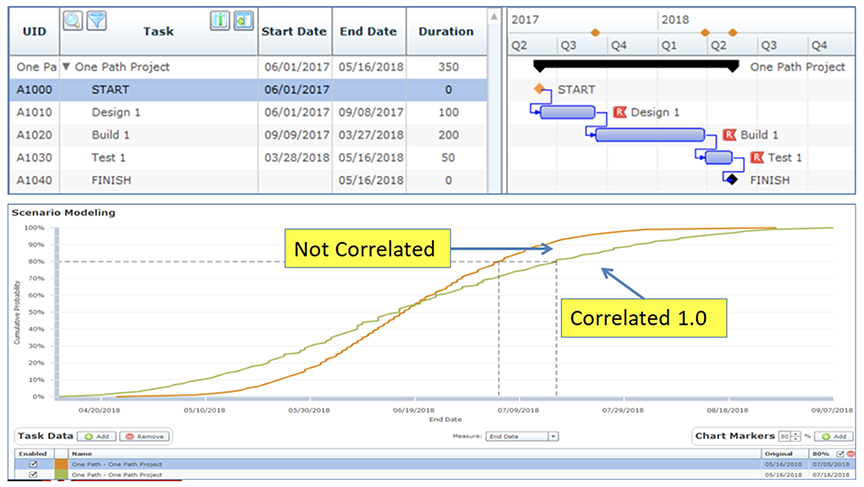
- Sometimes the analyst specifies correlation between activity durations. However, individuals are particularly ill-equipped to specify these correlations directly, having little information or experience on which to base the size of these coefficients. The effect of correlation can impact the projected finish date and probability of overrunning the scheduled date as shown in Figure 7. In that figure, all activities’ durations are either independent (“not correlated”) or 100% positively correlated (“Correlated 1.0”) with each other, pairwise. The scenario results differ significantly toward the ends of the distributions.
Figure 7: Effect of Correlation at 100% Imposed Directly on Activity Durations
7. LEVEL 4: MODERN QUANTITATIVE SCHEDULE RISK ANALYSIS MATURITY
7.1 Distinguishing Features at Level 4
The main capabilities available at maturity level 4 are gained because the Monte Carlo simulation is driven by (1) identified project-specific and systemic risks specified by their probability and impact and assigned to all activities they affect, and (2) uncertainty that is 100% likely, can be assigned as reference ranges by groupings of activities, and is of unknown origin so its impact on the finish date is unlikely to be reduced. These are shown in Figures 8 and 9.10 Figure 8 shows that uncertainty ranges based on inherent variability, estimating error and estimating bias, if any, may affect activities in groups of similar types such as engineering, procurement, etc.
Figure 8: Uncertainty Applied as Reference Ranges
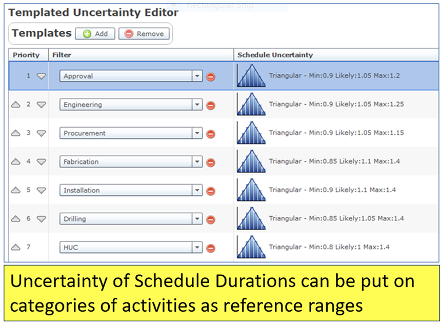
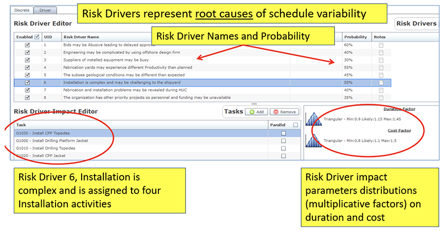
Figure 9 shows the set-up of several risk drivers with their (1) unique ID and name, (2) probability of occurring with some impact, (3) impact on duration (and cost in this case) expressed as distributions of multiplicative factors, and (4) activities they will affect, if they occur. Expressing the risks as multiplicative factors so that each iteration chooses a multiplier, if the risk occurs, that will be used to multiply the scheduled duration. The probability shown is implemented by having the risk occur on some percentage of the iterations. A probability of 70% implies that the risk will occur on a randomly selected 3,500 of the 5,000 iterations.
Figure 9: Identified Risks with Their Risk Parameters
The use of identified risks allows those risks to be assigned to many activities, if applicable, for the project. This also implies that some, perhaps many, activities are affected by more than one risk. These characteristics closely model the reality, particularly in complex projects, and produce benefits discussed later in this article.
When combined with the logical structure of the schedule, with parallel paths, merge points and critical paths, placing the influence of risks onto the right detailed tasks gives the result more accuracy and transparency.
7.2 Capabilities Required at Level 4
The risks have to be identified to be calibrated and to be modeled in the Monte Carlo simulation. Risk identification is required and discussed at level 2 where the risk register is first developed. Risk identification for quantitative risk analysis is needed at level 4. Usually the risk register is not complete so further risk data gathering is needed.
One difference from qualitative risk analysis at level 2 is that when the risks are applied to activities’ durations the impact measure is the range of making activity durations longer or shorter rather than level 2’s concept of the range of making the project finish date earlier or later. At level 4, the impact values affecting specific activities’ durations are clearer and simpler at a more detailed level and therefore easier for project team members to assess.
In addition, working with clients across multiple commercial and government sectors, risk data collection interviews find that the risk register is always incomplete. This is implied by the fact that risk information collected using confidential risk interviews, often a component of maturity level 4, discovers risks that are not in the risk register. Hence, enhanced methods of risk data collection are employed at level 4.
The risk analyst will often decide to develop a summary schedule for the risk analysis. Common contractor-developed schedules are not always compliant with scheduling best practices and, in any case, they contain more detailed activities than are needed in a strategic risk analysis.2 A summary schedule needs to include representation of all the work in the project according to the plan at the time of the analysis. The summary schedule’s paths should be visible and have similar total float values and linkages to other paths as in the detailed schedule.
7.3 Benefits/Strengths at Level 4
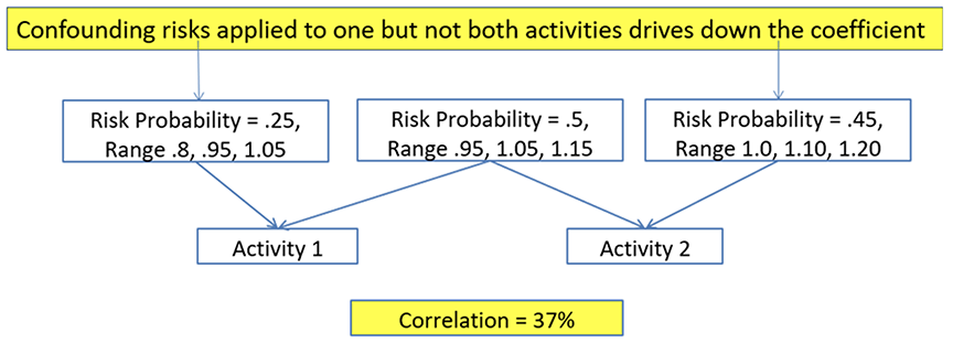
Using the project-specific and systemic risks to drive the simulation allows the analysis model to follow reality more closely than at level 3. In particular, the method used at this level of maturity known as risk drivers models how activity durations become correlated, removing the need for the analyst to estimate those values. Modeling correlations in this way also produces a correlation coefficient matrix that is nonnegative definite, i.e., have no negative eigenvalues.4 Modeling correlations and generating correlation coefficients during simulation is shown in Figure 10:
Figure 10: Modeling How Risks Affect Activities’ Durations
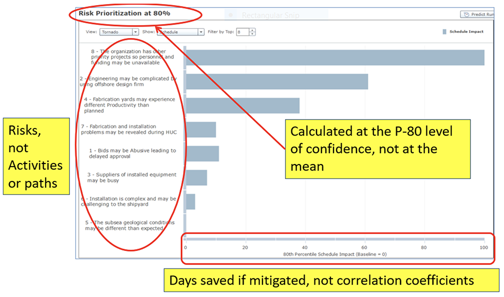
Since identified risks are used to drive the simulation, those risks can be prioritized: (1) by their marginal impact on the PRA results, (2) at a target level of confidence such as the P-80, and (3) by calibrating the risks’ priority order by days saved, if they were fully mitigated. This information is useful for project management to determine whether to implement mitigation so that its benefits in days saved are worth the cost of the mitigation actions proposed. This prioritization measure is better than traditional “tornado diagrams” expressed in activities rather than risks and using correlation of those activities with the finish date instead of days saved. The results of a risk prioritization using this method are shown in Figure 11.5
Figure 11: Risks Prioritized by Days Saved if Mitigated
7.4 Weaknesses at Level 4
Maturity level 4 exhibits the strengths derived from the use of uncertainty and identifiable risks that are lacking at level 3. One issue to confront is that some projects, often the smaller and shorter projects, do not have a project schedule to use. Sometimes the schedule available is not consistent with scheduling best practices. On occasion a summary analysis schedule needs to be built.
As with all of these Monte Carlo-based risk analyses (Levels 3 – 5) the main source of risk data is derived from individual project participants and other subject matter experts (SMEs) who have knowledge from their experience in the field and on other similar projects. They bring whatever data they may have as well as their knowledge of the specific project and in general. There are some cautions about this method of data collection.
Individuals are known to exhibit biases when discussing uncertainty concepts, which are about future events. An eminent statistician once said, “There are no facts about the future”12 so one needs to recognize their inherent biases and try to offset them.16 This is why confidential interviews are often used to put the interviewees in a safe environment where they can say what they really mean without fear of contradiction or unwanted repercussions. An expert interviewer can usually identify the biases in the interviewee’s responses and overcome or correct for them.
Still, there is a need to check the results from Monte Carlo simulation using individual risk data inputs against historical experience with similar completed projects. One approach to interrogating the historical data is to perform regression analysis on large databases specifically developed to illustrate the experience of executing projects against their planned cost and schedule. The analysis of the historical data typically examines the influence on cost and schedule results of systemic risks that tend to be present in large and complex projects. Systemic risks include:3, 9
- Completeness of scope definition
- Quality of project controls
- Quality of project scheduling
- Quality of team development
- Extent of new technology in the project
- Extent of complexity
This analysis of historical data brings the perspective of an “outside view.”6
8. LEVEL 5: ADVANCED INTEGRATED COST-SCHEDULE RISK ANALYSIS (ICSRA) MATURITY
This level of maturity recognizes the important fact that activity durations and costs are related. If the activity has labor-type resources, the costs will be higher if the task takes longer and the ICSRA approach is to model these cost increase in proportion to the extension of duration. Indirect costs can be placed on hammock activities and will react in proportion to the variation of the detailed activities supported. The project cost budget built on the schedule using resources should exclude a cost contingency because the MCS modeling approach will produce an estimate of cost contingency and should not double-count the contingency in the estimate.11
8.1 Distinguishing Features at Level 5
Level 5 builds on all the capabilities of level 4, including basing the analysis on the project schedule and using uncertainty and project-specific risks to drive the Monte Carlo simulation.
The distinguishing characteristic at level 5 is that the schedule is resources loaded with the costs, both direct and indirect, of the project without contingency having been applied. The resources are distinguished by being time-dependent (labor plus equipment rented by the day) and time‑dependent (material plus equipment to be installed and perhaps some subcontracts). Only the time-dependent costs respond to schedule variability. Resource use or “daily burn rate” for labor and total cost for materials may be affected independent of schedule variability because of typical cost-risk variables like uncertain labor rates or world price of materials.
8.2 Capabilities Required at Level 5
Often the project schedule is not loaded with resources or those resources are not associated with cost categories matching the budget. To place the costs by resources on the schedule activities the cost estimators and the schedulers need to communicate at a common detailed level using the same Work Breakdown Structure (WBS). This communication is not always easy since the estimate and schedule may have diverged and be using incomplete or incompatible WBS.
8.3 Benefits/Strengths at Level 5
The Monte Carlo simulation will compute the cost that is related to the schedule result for each iteration. A consistent pair of finish dates and cost is calculated, both reflecting the effects of uncertainty and risk for any iteration. The costs that result will be affected by that iteration’s assumptions. In this way, the cost and finish date results would be computed for the same project (structure and risks) in the iteration. Each iteration could be the project’s results, but the analyst can only make statistical statements about the probability of a finish date being earlier or later than a particular date.
The analysis does not identify which party must pay for the extra costs. Depending on the contract, there may be a presumption that the owner or the contractor pays the cost. Of course, there may be compensable reasons for the work to have taken longer and in making claims the owner may pay some or all of the cost even with a lump-sum turn-key contract.
Histograms for schedule are the same as at level 4. Histograms for cost reflect both the indirect effect of schedule risks on activity durations with time-dependent resources and cost-risks on labor’s burn rate and on time-independent resources.
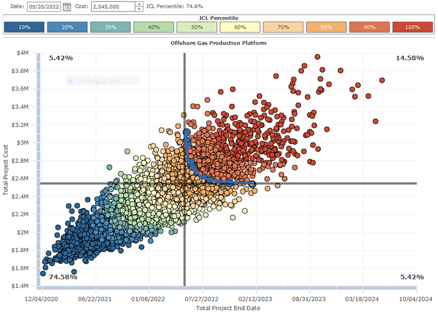
A new concept of project risk is available from the integration of cost and schedule at maturity level 5. This is the concept of providing estimates of finish date and total project cost that have a joint probability of both occurring at some percentile. This concept is needed because given the P-80 confidence level for schedule and cost separately there are results for the other objective that do not have a P-80 chance of being met. To look at finish date and cost that both finish at the P-80 (or whatever certainty level is desired), the analyst has access to a scatter diagram.
What this joint probability of cost and schedule does is to allow the analyst to choose a combination of finish dates and costs that have, for example, an 80% likelihood of success with both objectives. Finding the dates and costs where both cost and schedule are 80% likely to succeed will generally require a later finish date and higher project cost than those found using the typical histogram P-80 values for cost and finish date separately.
This is shown by using the scatterplot shown in Figure 12. There the P-80 time and cost from histograms and cumulative distributions for cost and finish date derived from the simulation separately but not shown, are indicated by the cross-hairs in Figure 12. The scatterplot shows that in this case there is only a 74.6% probability of both occurring (i.e., 74.5 % of all iteration scenarios or 3,730 of the 5,000 iterations are in the lower-left quadrant from that point).
Figure 12: The P-80 Values for Cost and Finish Date
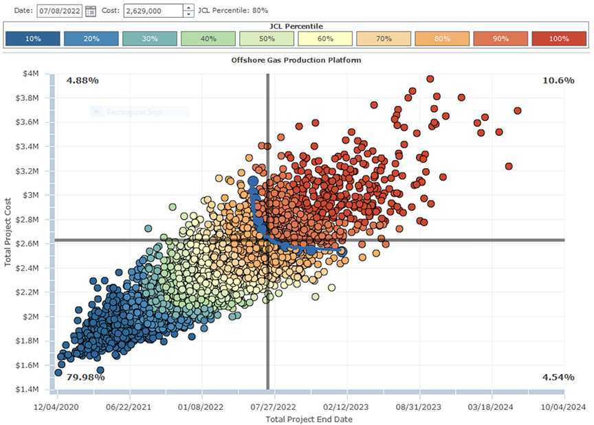
Looking at both cost and schedule together in Figure 12, the values of cost and finish date both need to be increased to meet on the line indicated by the iteration results connected blue dots. Anywhere on that necklace of blue dots will yield an estimate and finish date forecast that has an 80% chance of meeting both objectives. As can be seen, the target values for cost and finish date need to move in a north-easterly direction to meet the blue dots. This movement, toward a joint cost and finish date success, shown in Figure 13, will imply a later date and higher cost than those resulting from the separate histogram and cumulative distribution of time and cost.
Choosing the most likely point on the linked blue dots needs to be done for an 80% joint cost and schedule confidence level (JCL-80) forecast. The term “JCL” is the NASA term for this analysis.13 NASA requires the larger projects to implement JCL and uses a 70% target JCL level.
The most likely values would be found on the scatter diagram where the iterations are most heavily concentrated. Figure 13 shows one such likely point. The JCL-80 point chosen is July 8, 2022 which is about 7 weeks later than the P-80 finish date and $2.629 billion, which is about $84 million above the P-80 cost. Specifying this date is done by finding the most likely JCL-80 date and cost, staying in the part of the scatterplot where the results are most dense.
The added cost and schedule days allows management to specify a budget and finish date that are both likely to meet the desired confidence level.
Figure 13: Selecting a JCL-80 Cost and Finish Date Target
8.4 Weaknesses at Level 5
The weaknesses at level 4 are present at level 5.
In addition, there is an unresolved issue in picking the specific cost and finish date that is the most likely combination to provide a probability of both achieving both cost and finish date targets at the chosen JCL level of confidence. Figure 13 shows a combination chosen to be in the area of the scatterplot where the simulation results are most concentrated. Such a point would be the most likely combination that provides the desired level of confidence. If the scatterplot were viewed as a 3‑dimensional ridge of possible results, this point would be the one on the necklace of connected dots with the desired joint success result. The problem is that at this point the choice of a JCL combination of cost and finish dates is judgmental to some extent. While uncertainty in the single most likely JCL point with desired joint success probability properties would be expected in a statistical analysis, some users, including reports to Congress for funding or to the board of directors, may require choosing single-point precise values. One approach to improving the accuracy of finding the most likely JCL combination has been offered at a recent NASA cost‑schedule symposium.21
9. CONCLUSION
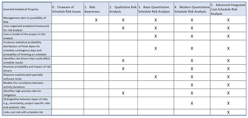
The levels of schedule risk analysis maturity in project management ranging from no awareness to fully integrated cost-schedule risk analysis have been described with their capabilities required, benefits and strengths and weaknesses at a general level. Illustrations are given for the main inputs and outputs at levels 2–5. A summary is show in Table 1 for the main characteristics of risk maturity levels.
Table 1: Summary of Key Characteristics by Risk Maturity Level
About the Author
David T. Hulett, Ph.D., FAACE, is a Cost & Schedule Risk Analysis Partner affiliated with Long International. He has conducted many risk analyses, focusing on quantifying the risks and their implications for project cost and schedule, and many schedule assessments. Dr. Hulett is a Principal with Hulett & Associates, LLC (H&A), and has focused for nearly 30 years on quantitative schedule risk analysis, integrated cost-schedule risk analysis, and project scheduling best practices. H&A clients are in oil and gas, aerospace, construction, pharmaceuticals, and transportation. They are located in the U.S., Canada, South America, Southeast Asia, Europe and the Middle East. H&A has pioneered the Risk Drivers approach to schedule risk and integrated cost and schedule risk analysis and he has recommended adopting this method for new and emerging Monte Carlo software to serve the needs of his high-end risk analysis customers. Dr. Hulett has experience in applying Risk Drivers to large multi-year projects leading to proactive risk mitigation planning for better project results. From these analyses, the client learns: the probability of achieving the cost and schedule with the existing project plan, the amount of time and cost contingency required to achieve a desired level of certainty, which priority risks drove the analysis results, and which risk mitigation actions address the risks. Dr. Hulett is based in Los Angeles, California and can be contacted at dhulett@long-intl.com and (310) 476-7699.
REFERENCES
1 AACE International, “Contingency Estimating – General Principles,” Recommended Practice 40R-08, AACE International, Morgantown, WV (2008 or latest revision).
2 AACE International, “Integrated Cost-Schedule Risk Analysis using Monte Carlo Simulation of a CPM Schedule,” Recommended Practice 57R-09, AACE International, Morgantown, WV, (2011a or latest revision).
3 AACE International, “Risk Analysis and Contingency Estimating using Parametric Estimating,” Recommended Practice 42R-08, AACE International, Morgantown WV, (Rev. 2011b or latest Revision).
4 Book, Stephen A., “A Theory of Modeling Correlation for Use in Cost-Risk Analysis,” Third Annual Project Management Conference, NASA, 2006.
5 Druker, Eric, Graham Gilmer and David Hulett, “Using Stochastic Optimization to Improve Risk Mitigation,” AACE International Annual Conference, 2015.
6 Flyvbjerg, Bent, “From Nobel Price to Project Management: Getting Risks Right,” Project Management Journal, Vol. 37, No. 3, pp. 5–15, Project Management Institute, 2006.
7 GAO, Schedule Assessment Guide: Best Practices for Project Schedules, GAO-16-89G, Government Accountability Office, 2015.
8 Hollmann, John K., “Risk.1027, Estimating Accuracy: Dealing with Reality,” Transactions, AACE International, 2012.
9 Hollmann, John K., Project Risk Quantification, Probabilistic Publishing, 2016.
10 Hulett, David T., Practical Schedule Risk Analysis, Gower Publishers, 2009.
11 Hulett, David T., Integrated Cost-Schedule Risk Analysis, Gower Publishers, 2011.
12 Moses, Lincoln, Administrator of the Energy Information Administration, 1979 Annual Report to Congress, DOE/EIA-0173 (79) / 3, US Department of Energy, 1979.
13 NASA, Cost Estimating Handbook, Appendix J Joint Cost and Schedule Level (JCL) Analysis, National Aeronautics and Space Administration, 2015.
14 Project Management Institute, A Guide to the Project Management Body of Knowledge (PMBOK®) Guide, Fifth Edition, Project Management Institute, 2013.
15 Project Management Institute, A Guide to the Project Management Body of Knowledge (PMBOK®) Guide, Sixth Edition, Project Management Institute, 2017.
16 Tversky, Amos and Daniel Kahneman, “Judgment under Uncertainty: Heuristics and Biases,” Science, New Series, Vol. 185, No. 4157, (Sep. 27, 1974).
17 Wikipedia, “There are Known Knowns,” from Donald Rumsfeld, Secretary of Defense, https://en.wikipedia.org/wiki/There_are_known_knowns, cited 12/24/2017.
18 Hillson, David, Effective Opportunity Management for Projects, Exploiting Positive Risk, Marcel Dekker, Inc., 2004
19 MacCrimmon, Kenneth and C. A. Ryavek, “An Analytical Study of the PERT Assumptions,” Research Memorandum RM-3408-PR, Rand Corporation, 1962.
20 AACE International, Risk Assessment: Identification and Qualitative Analysis, Recommended Practice 62R-11, AACE International, Morgantown, WV (2012 or latest revision).
21 Steiman, Sam and David Hulett, “Identifying the Most Probable Cost – Schedule Values from a Joint Confidence Level (JCL) Analysis,” NASA Cost and Schedule Symposium, Goddard Space Flight Center August 14-16, 2018.
Republished with the permission of AACE International, 1265 Suncrest Towne Centre Dr., Morgantown, WV 26505 U.S.A.
Telephone: +1 (304) 296-8444 | Facsimile: +1 (304) 291-5728 | web.aacei.org | Email: info@aacei.org
Copyright © 2018 by AACE International | All rights reserved
ADDITIONAL RESOURCES

Articles
Articles by our engineering and construction claims experts cover topics ranging from acceleration to why claims occur.
MORE

Blog
Discover industry insights on construction disputes and claims, project management, risk analysis, and more.
MORE

Publications
We are committed to sharing industry knowledge through publication of our books and presentations.
MORE