ABSTRACT – Monte Carlo simulations are often used in cost estimating to calculate the proper contingency required to address a project’s risks and uncertainties, yet this tool is seldom employed past the estimating phase. However, the use of Monte Carlo simulations is just as applicable in calculating uncertainties in the dispute resolution and claims process, whether in assessing a Contractor’s most-likely claim recovery or exposure for use in negotiations, or ranging the cost impact of missing, incomplete, or disparate data when preparing a claim.

This paper provides a brief overview of the mechanics of Monte Carlo simulations, outlines potential applications in the dispute resolution and claims process, and provides examples from real world projects. The intent is to provide contractors, owners, attorneys, and consultants with an additional tool to assess and better calculate the risks and uncertainties in the claims process.

Keywords: Claims, contingency, dispute resolution, estimating, projects, and risk

RISK AND UNCERTAINTY IN CONSTRUCTION DISPUTES

The claims resolution process, starting with a project dispute and ending through negotiation, mediation, arbitration, or trial is filled with uncertainty. The contractor, which may have sustained substantial losses on the project, prepares a claim document, but may not have the necessary records, resources, methods, or time to fully delineate all issues and prove its recoverable damages. The owner then evaluates the claim, assessing large and complex issues with sometimes limited or incomplete data, especially related to the contractor’s records. During negotiations or mediation, either party can easily underestimate or overestimate the relative strength of its position. And there is certainly risk in taking the dispute to arbitration or trial, where an arbitrator, jury, or judge can take a different position than anticipated by either party.

MONTE CARLO SIMULATION APPLICATIONS

Monte Carlo risk simulation is one tool that can help parties better evaluate, quantify, and understand the uncertainty and risk present in a given situation. Simulations are typically performed with relatively inexpensive software¹ and provide probabilistic outcomes, i.e., a range of results with different likelihoods, rather than a single-value (or deterministic) result.

A spreadsheet model is prepared in which user-defined ranges are applied to a set of variables, those items or issues which are not known with certainty. In a given trial, Monte Carlo Simulations assign a random number within the user-defined range for each variable and calculate a result. The results, after thousands of trials, are plotted in a probabilistic curve which shows not only the most likely outcome, but also a range of possible outcomes, and the probability of those outcomes. If performed correctly, the simulations are a cost-effective way to provide additional, accurate data relative to an owner’s or contractor’s risks. The simulations remain estimates whose accuracy is defined by user inputs, but the results are more functional than other single-point estimates that may be produced.

In the authors’ experience, Monte Carlo Simulations are most effective early in the claims process, when attempting to settle disputes through negotiation or mediation, or to help guide case strategy. As the dispute progresses to arbitration or litigation, uncertainty with respect to many issues should decrease simply because additional information becomes available through discovery, witness interviews, depositions, and further detailed analyses. Estimating uncertainty, then, becomes less important. Furthermore, while expert reports often include estimates related to the Contractor’s or Owner’s quantum, the probabilistic curves created using Monte Carlo Simulations can be seen as less definitive than single-point estimates, and therefore they are likely more subject to criticism. This should not preclude an expert from using Monte Carlo Simulations in cases where it may be necessary, but their use in an expert report would be highly dependent on the venue and the comfort level of the expert with such an approach.

This paper outlines two examples where Monte Carlo Simulations were utilized early in the claims process. The first shows how Monte Carlo can be used to assess a Contractor’s most likely claim recovery. The second demonstrates how a Monte Carlo Simulation was employed to estimate un‑expedited construction costs to settle an insurance dispute.

CLAIM ASSESSMENTS

One useful application of Monte Carlo Simulations is to assess a party’s likely claim value recovery. Table 1 shows an Owner’s breakdown of a Contractor’s $33 million claim into six major components, and a breakdown of its $6.5 million counterclaim into two components.

Table 1 – Claim Assessment ($Millions)

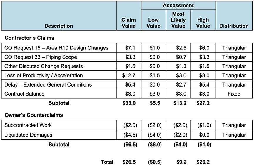
Without using a Monte Carlo Simulation, the Owner’s risk assessment may be confined to a few values based upon limited scenarios. Table 1 shows that the Owner has calculated the Contractor’s most likely recovery net of the Owner’s counterclaims as $9.2 million, with the Owner’s best case being a recovery from the Contractor of $0.5 million and its worst case being a payment to the Contractor of $26.2 million. The results include a wide range of risk with no indication of the probability of any outcome.

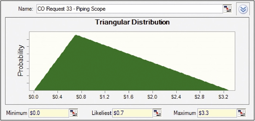
These same low, most likely, and high values can be used as ranges in Monte Carlo Simulations using a common distribution format, triangular distribution.² The recovery related to Change Order Request 33, for example, would be modeled using the triangular distribution shown in Figure 1. Based upon the user-defined ranges, the Monte Carlo Simulation selects a number for each trial ranging from $0 to $3.3 million, with $0.7 million being the most likely selection.

Figure 1 – Triangular Distribution Example

With each claim component similarly distributed within the ranges shown in Table 1, the resulting probabilistic outcomes of the Monte Carlo Simulation, based upon 10,000 trials, are shown in Figure 2.

Figure 2 – Probability Curve of Contractor’s Recovery Value

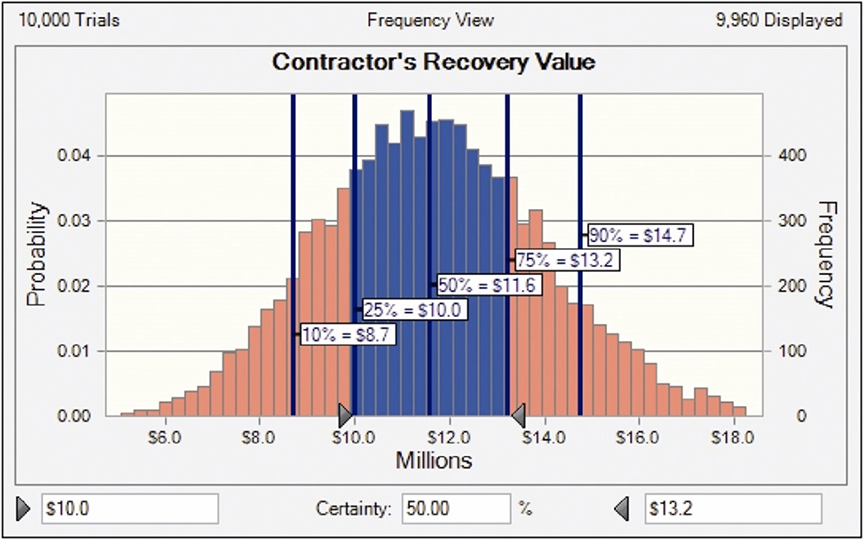
The results from the Monte Carlo Simulation indicate that the median value is $11.6 million, with 50 percent of all trials falling between $10.0 million and $13.2 million. Further, 80 percent of all trials fell between $8.7 million and $14.7 million.

Comparing the probabilistic results of the Monte Carlo Simulation with the deterministic values provided in Table 1, the following are observed:

• The most likely recovery value in the deterministic model, $9.2 million, increased to a median³ (P50) value of $11.6 million in the simulation. In effect, the uncertainty of the high-range values in the Monte Carlo Simulation significantly increased the most likely outcome.
• The range of probable outcomes decreased substantially. The Owner’s best and worst case scenarios ranged from a $0.5 million recovery to a $26.2 million payment. With the user-defined assumption included in the Monte Carlo Analysis, some 80 percent of the trials fell within only a $6.0 million range.

The result of the Monte Carlo Simulation, assuming accurate inputs, provides the Owner with a more accurate most likely outcome, as well as a better-defined range of outcomes to approach settlement negotiations. As with any computer model, the accuracy of the results depends upon the accuracy of the user-defined inputs. In this and all cases, the analysts must ensure that the defined ranges and distribution models are consistent with the uncertainty present at the time.

This example represents a simple claim assessment that might be made early in the review process, when limited supporting data and documentation has been provided or reviewed. The models can be made much more complex, and accurate, as the claim assessment process develops. For example, each claim category can be ranged from an entitlement perspective, using input from attorneys and/or technical experts, as well as a damages perspective, wherein the claim calculations are assessed based upon the data presented and the methodology employed.

Assume in this case that the Contract for the Project included a “no damages for delay” clause. Clearly, the arbitrators’ decision relative to this clause would impact the Contractor’s recovery of its $5.4 million delay claim. Table 2 shows how this uncertainty could be modeled in the Monte Carlo Simulation.

Table 2 – Delay Claim Assessment ($Millions)

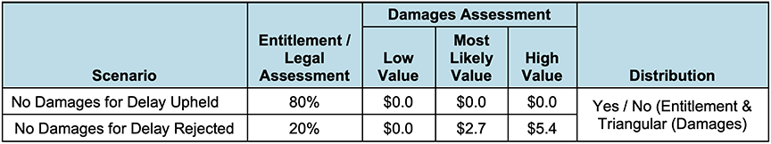
Based upon input from the Owner’s attorneys, the model includes an 80 percent likelihood that the “no damages for delay” clause would be upheld by the arbitrators. In the Monte Carlo Simulation, approximately 80 percent of the trials would result in no recovery for the Contractor. In the remaining 20 percent of the trials, the Contractor’s recovery would be ranged based upon the triangular distribution previously discussed.

Disputed change order requests might be similarly assessed from an entitlement standpoint to determine if the claimed additional work was part of the Contractor’s original scope. Again, percentages could be included in the model based upon the confidence of prevailing on each issue, with the calculation of change order costs assessed separately.

A further feature that should be included in every model relates to the correlation of variables, or in this case, the inter-relationship between claim components. Without correlation, each trial in a Monte Carlo Simulation is random within the given ranges. That means, returning to Table 1, that the simulation could include a trial wherein the contractor’s delay claim recovery is $5.4 million while the Owner’s recovery for liquidated damages is $4.5 million. The arbitrators’ decision would never include such an occurrence; if the Contractor were to recover its full claim relative to delay, the Owner would likely receive no liquidated damages, with the inverse being true as well. Therefore, it is necessary for the model to include the appropriate correlation between claim components, which is easily accomplished with most Monte Carlo Simulation software.⁴

Whether a simple or more sophisticated model is utilized, Monte Carlo risk simulation can provide an owner or contractor invaluable information to better negotiate a claim settlement, assess potential recovery or exposure in arbitration or litigation, and set an effective claim strategy to manage legal and consulting tasks and costs.

NEGOTIATED COST ESTIMATE

Monte Carlo Simulations are extremely valuable in resolving complex disputes where many issues are uncertain. The dispute in this example involved the rebuild of a facility damaged by fire. Two insurance underwriters were involved: Insurance Company A provided property damage coverage to pay for the costs of the rebuild, and Insurance Company B provided business interruption insurance. Construction was performed on an expedited basis involving significant manpower, overtime, and shift work to get the facility back online quickly. The expedited work was beneficial to Insurance Company B, as it minimized the business interruption costs, but detrimental to Insurance Company A, because construction costs increased. Insurance Company A sought an equitable adjustment from Insurance Company B related to the expediting costs.

As the insurance companies entered negotiations, cost consultants for both companies were tasked with calculating the un-expedited costs of construction. This meant assessing installed quantities, unit productivity rates, manpower, overall schedule duration, overhead costs, and other costs, all of which had a degree of uncertainty. The assessment was similar to that which would be done by a Contractor bidding the work, but in this case, two parties with differing interests had to agree with the estimate.

A Monte Carlo Simulation was used to perform the cost estimate. The Contractor’s quantity, man-hour, and cost records related to construction were available, but the data was found to be somewhat incomplete and not fully reliable. For instance, installed quantities were calculated using vendor invoices and as-built drawings, but were ranged to account for incomplete data. Similarly, the Contractor’s actual unit labor productivity rates for each discipline were considered, as were unit productivities achieved for past projects in the area as well as productivities from industry manuals. All productivities were normalized for un-expedited work in the region.

Table 3 – Range Data – Electrical

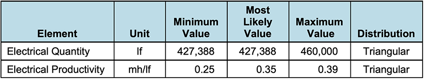
Quantity and labor productivity data were ranged using minimum, maximum, and most likely values so that a triangular distribution could be utilized. The range data for electrical work is shown in Table 3. Once quantity and productivity data were ranged for each discipline, a Monte Carlo Simulation was used to calculate the probability curve for total labor man-hours, as shown in Figure 3.

Figure 3 – Probability Curve of Total Estimated Man-Hours

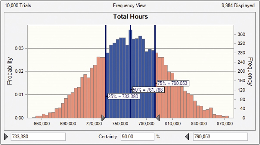
After the total man-hours were modeled, the analysts turned to the assessment of project duration. The end date of the project had to be known in order to estimate the Contractor’s overhead costs. Moreover, working in an un-expedited basis, the Project duration could potentially extend into additional winter months, which would further impact direct labor productivity. Given the man-hour distribution in Figure 3, the task was to determine the distribution of project end dates.

Figure 4 illustrates the model that was developed to simulate the Contractor’s manpower for several different phases of the Project. Rectangles and triangles were used for simplicity such that spreadsheets could be developed to calculate areas, which were in turn used to calculate durations and end dates.

Figure 4 – Model of Project Manpower

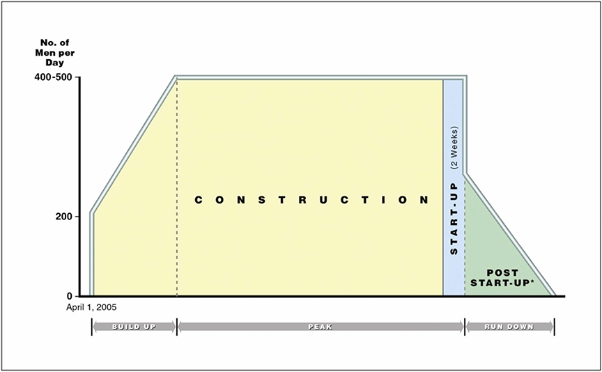
Peak manpower was another area of uncertainty and, therefore, became a variable which was ranged in the analysis. These ranges were developed based upon the Contractor’s actual manpower during the project, crowding studies, and negotiations between the parties.

In each trial, the Monte Carlo Simulation performed the following series of calculations to determine an end date:

• Selected quantity and unit productivity values from the user-defined ranges for each discipline;
• Calculated total man-hours based upon quantity and productivity selections;
• Selected a peak manpower value within the user-defined range; and
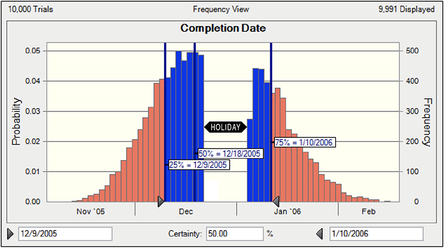
• Calculated the project duration and end date based on the calculated total man-hours and selected manpower. After 10,000 trials, the Monte Carlo Simulation provided the end date distribution shown in Figure 5.

Figure 5 – Probability Curve of the Project Completion Date

The estimate was completed by applying the appropriate costs, some of which were ranged, to the modeled quantities, man-hours, and project durations. The result of the Monte Carlo Simulation was a probability curve showing the total estimated costs, similar to the man-hour curve shown in Figure 3, which the authors understand was used to negotiate an equitable settlement between the insurance companies.

In all, more than 25 separate variables were ranged and incorporated into a relatively sophisticated spreadsheet model. Monte Carlo Simulation is most valuable with these complex models because it performs numerous calculations quickly and provides a probabilistic range of results. In addition, the variables, or ranged elements, in Monte Carlo Simulations can be tested to determine their sensitivity, which indicates the magnitude that an element has on the final outcome.

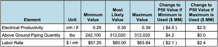
Table 4 shows the three most impacting elements on the Monte Carlo Simulation. If, for example, the most likely labor rate was chosen to be $57.25 per hour rather than the $60.00 per hour used, the median (P50) value of the estimate would have decreased by $2.1 million. The analysts must review these sensitivities to ensure that the analysis is balanced, and that no one element is driving the results (unless it should be).⁵

Table 4 – Example Sensitivity Analysis – Top 3 Elements

In this case, once the variable ranges were assessed, negotiated, and agreed, the final cost estimate was less subject to scrutiny. An appropriate question to ask is how this dispute would have been settled without using a Monte Carlo Simulation. The parties would have had to agree to one value for each of 25 variables, which would have resulted in one value for the final un-expedited costs. While negotiations could have started from that point, it is clear that the probabilistic results from the Monte Carlo Simulation provided more useful data for negotiations.

About the Authors

Rod C. Carter, CCP, PSP, is President of Long International, Inc. He has over 20 years of experience in construction project controls, contract disputes and resolution, mediation/arbitration support, and litigation support for expert testimony. He has experience in entitlement, schedule, and damages analyses on over 30 construction disputes ranging in value from US$100,000 to US$7 billion, related to oil and gas, heavy civil, nuclear, environmental, chemical, power, industrial, commercial, and residential construction projects. He is proficient in the use of Primavera Project Planner software and has extensive experience in assessing the schedule impact of RFIs, change orders, and other events to engineering and construction works. Mr. Carter specializes in loss of productivity, cumulative impact, and quantum calculations, and has held a lead role in assessing damages on more than a dozen major disputes. In addition, Mr. Carter has developed cost and schedule risk analysis models using Monte Carlo simulations to address the uncertainty of estimates and claims. He has testified as an expert in construction scheduling and damages and has presented expert findings to an international arbitral tribunal. Mr. Carter earned a B.S. in Civil Engineering from the University of Colorado at Boulder in 1996, with an emphasis in Structural Engineering and Construction Management. Mr. Carter is based in Littleton, Colorado, and can be contacted at rcarter@long-intl.com and (303) 463-5587.

Richard J. Long, P.E., P.Eng., is Founder of Long International, Inc. Mr. Long has over 50 years of U.S. and international engineering, construction, and management consulting experience involving construction contract disputes analysis and resolution, arbitration and litigation support and expert testimony, project management, engineering and construction management, cost and schedule control, and process engineering. As an internationally recognized expert in the analysis and resolution of complex construction disputes for over 35 years, Mr. Long has served as the lead expert on over 300 projects having claims ranging in size from US$100,000 to over US$2 billion. He has presented and published numerous articles on the subjects of claims analysis, entitlement issues, CPM schedule and damages analyses, and claims prevention. Mr. Long earned a B.S. in Chemical Engineering from the University of Pittsburgh in 1970 and an M.S. in Chemical and Petroleum Refining Engineering from the Colorado School of Mines in 1974. Mr. Long is based in Littleton, Colorado and can be contacted at rlong@long-intl.com and (303) 972-2443.

References:

¹     Figures 1 through 4 presented in this paper were prepared using Crystal Ball^® software.

²     Triangular distribution is one of several distributions available in Monte Carlo Simulations and is typically employed when minimum, maximum and most likely values are known or can be reasonably estimated. Other commonly used distributions include uniform, normal, and beta.

³     The median value is often referred to as the P50 value, the point at which 50 percent of all trials fall below the value. The median value does not always represent the most-likely value.

⁴     Crystal Ball^® software, for example, provides a drop down menu where a correlation coefficient can be selected between any two variables, with a 0 denoting no correlation and 1 denoting full correlation between variables.

⁵     Sensitivity is also used to identify the element or elements with the largest uncertainties and impacts. In the prior example related to the assessment of a Contractor’s claim, the sensitivity analysis could be used to determine which claim elements to focus on, if it is not obvious from the magnitude of the claimed costs.

Originally published by AACE International as CDR.10 in the 2009 AACE International Transactions.
Reprinted with the permission of AACE International, 1265 Suncrest Towne Centre Dr., Morgantown, WV 26505 U.S.A.
Telephone: +1 (304) 296-8444 | Facsimile: +1 (304) 291-5728 | Internet: web.aacei.org | Email: info@aacei.org
Copyright © 2009 by AACE International; all rights reserved.