ABSTRACT

AACE® International’s Recommended Practice No. 29R‑03 for Forensic Schedule Analysis (RP 29R‑03) presents nine different methodologies for performing schedule analyses. Some schedule analysis methods are better suited for certain purposes than others. Each method is unique in its applicability to a given set of project specifics, including: type of project, legal jurisdiction, contract documents, dispute resolution mechanism, fact pattern, and other project execution factors. A mismatch between project specifics and the selected methodology can substantially undermine a party’s chance of recovery, add unnecessary costs, and distract from factual entitlement issues.

Familiarity with the key elements of AACE® 29R‑03 and a clear understanding of the core assumptions, strengths and weaknesses of the recommended methodologies is a basic, yet critical, step for properly implementing a schedule analysis. This paper presents an overview of each of the nine schedule analysis methodologies, the nomenclature used to categorize the different methods, and the strengths and limitations of each method. It then discusses eleven factors a forensic schedule analyst should consider when choosing the most appropriate schedule analysis method.

1.    INTRODUCTION

AACE® International’s Recommended Practice No. 29R-03 for Forensic Schedule Analysis (RP 29R‑03) was initially published on June 25, 2007, and subsequently revised on June 23, 2009 and April 25, 2011. RP 29R‑03 presents nine different methodologies for performing schedule analyses and discusses eleven technical, legal, and practical factors for consideration when choosing a forensic schedule analysis methodology. The primary purpose of RP 29R‑03 was to foster competent schedule analysis and furnish the industry as a whole with the necessary technical information to categorize and evaluate the varying forensic schedule analysis methods.

This paper presents an overview of each of the nine schedule analysis methodologies, the nomenclature used to categorize the different methods, the strengths and limitations of each method, and eleven factors to consider when choosing the most appropriate schedule analysis method. The graphics and concepts discussed in this paper are sourced, excerpted, and/or paraphrased from RP 29R‑03 with permission from AACE. The purpose of this paper is to introduce to individuals unfamiliar with RP 29R‑03 the nine different schedule analysis methodologies and eleven factors to consider when choosing a forensic schedule analysis methodology, as well as to suggest potential improvements to RP 29R‑03.

The legal industry immediately perceived the significance of AACE® 29R‑03, and construction law firms, such as Watt Tieder, commented on it in regards to reconciling technical and legal factors when choosing a forensic schedule analysis methodology.¹ Also, in June 2015, Harold D. Lester, Jr., Board Judge, presided over Yates-Desbuild Joint Venture’s (YDJV’s) Motion to exclude the testimony of the U.S. Department of State’s scheduling expert witness, as well as the entirety of his expert report, because his methodology was allegedly flawed and not recognized in the industry.² YDJV’s Motion was based on the assertion that the U.S. Department of State’s scheduling expert’s methodology was flawed and was not recognized in the industry because: 1) it was not supported by RP 29R‑03 and 2) his analysis was inconsistent with RP 29R‑03.

Judge Lester denied the motion but did not object to the use of RP 29R‑03 by the moving party.  Neither did Judge Lester dismiss the Motion as frivolous. That the attorneys of Bradley Arant Boult Cummings LLP believed that strict non-compliance with RP 29R‑03 could be legitimate grounds for exclusion of an expert witness’ testimony highlights how far the recognition of RP 29R‑03 has progressed in the legal arena.

2.    FORENSIC SCHEDULE ANALYSIS TAXONOMY AND NOMENCLATURE

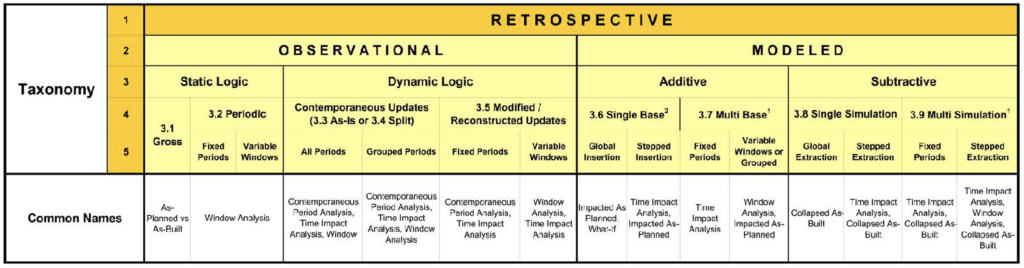
The foundation of AACE® 29R‑03 is a descriptive taxonomy, meaning a classification into ordered categories, of CPM-based schedule analysis methodologies. Figure 1 presents a summary chart of the RP 29R‑03 taxonomy. RP 29R‑03 focuses on retrospective schedule analyses, where the impacts of actual delays are known and can be quantified because they have already occurred. In contrast, prospective schedule analyses are based on the expected impacts of forecasted delays, changes, and/or added work scopes that have not yet occurred and not been fully documented.

Retrospective schedule analyses can be grouped into either observational or modeled methods. Observational schedule analysis methods involve examining a schedule without the analyst making revisions to the schedule to simulate a specific scenario. Modeled schedule analysis methods require the analyst to insert or remove delay events into or from a Critical Path Method (CPM) network to compare the calculated results of the “before” and “after” conditions.

Figure 1 : Nomenclature Correspondence
(Reprinted with permission of AACE® International) [ 1, page 12 ]

3.    NINE METHOD IMPLEMENTATION PROTOCOLS

The RP 29R‑03 taxonomy identifies nine Method Implementation Protocols (MIP’s) for forensic schedule analysis which are summarized below.

3.1    OBSERVATIONAL / STATIC / GROSS

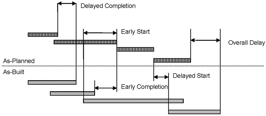
MIP 3.1 is an observational technique that compares the as-planned schedule to the as-built schedule. “In its simplest application, the method does not involve any explicit use of CPM logic and can simply be an observational study of start and finish dates of various activities. It can be performed using a simple graphic comparison of the as-planned schedule to the as-built schedule. A more sophisticated implementation compares the dates and the relative sequences of the activities and tabulates the differences in activity duration, and logic ties and seeks to determine the causes and explain the significance of each variance. In its most sophisticated application, it can identify on a daily basis the most delayed activities and candidates for the as-built critical path.” [ 1, pages 38-39 ]. Figure 3 presents the MIP 3.1 comparison of an as-planned and as built schedule and identifies activity start and completion delays and the overall project delay.

Figure 3 
Observational, Static, Gross Analysis Method
(Reprinted with permission of AACE® International) [ 1, page 38 ]

MIP 3.1 has been generally deemed unsuitable for the following situation:

• Project durations extending into multiple dozens of update periods.
• Projects built in a manner significantly different than planned.
• Complicated projects with multiple critical paths.
• Projects with several critical path changes.
• Projects with concurrent delays and pacing issues.

3.2    OBSERVATIONAL / STATIC / PERIODIC

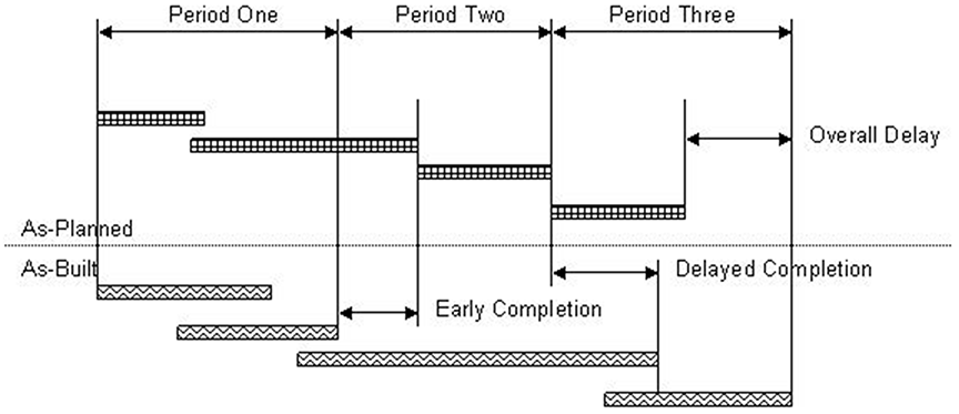
“Like MIP 3.1, 3.2 is an observational technique that compares the baseline or other planned schedule to the as-built schedule or a schedule update that reflects progress. But, this method analyzes the project in multiple segments rather than in one whole continuum.” [ 1, page 44 ]. “The advantage of performing this analysis in two or more time periods is that the identification of delays or accelerations can be more precisely identified to particular events.” [ 1, page 45 ]. “The fact that the analysis is segmented into periods does not significantly increase or decrease the technical accuracy of this method when compared to MIP 3.1.” [ 1, page 45 ]. Figure 4 presents the MIP 3.2 comparison of an as-planned and as built schedule divided into three periods.

Figure 4 
Observational, Static, Periodic Analysis Method
(Reprinted with permission of AACE® International) [ 1, page 44 ]

MIP 3.2 and MIP 3.1 share the same limitations.  MIP 3.2 “provides [ the ] illusion of greater detail and accuracy compared to MIP 3.1 where none exists…” [ 1, page 50 ].

3.3    OBSERVATIONAL / DYNAMIC / CONTEMPORANEOUS AS-IS

MIP 3.1 and 3.2 are static in the sense that they do not track the evolution of the critical path over time. MIP 3.3, on the other hand, “uses the project schedule updates to quantify the loss or gain of time along a logic path that was or became critical and identify the activities responsible for the critical delay or gain.” [ 1, page 51 ]. “[ I ]t relies on the forward-looking calculations made at the time the updates were prepared.” [ 1, page 51 ]. MIP 3.3 observes the activity dates and logic between update data dates, thus the concept of periods or “windows.” It also relies on schedule updates as prepared contemporaneously during the project execution, “based on essentially unaltered, existing schedule logic.” [ 1, page 51 ].

Limitations of MIP 3.3 include:

• MIP 3.3 is only as accurate as the contemporaneous schedule updates it relies upon. The updates must be validated; if they require significant modification (date constraints, relationships, durations, progress data) to accurately reflect both reported progress and means and methods, then MIP 3.3 becomes MIP 3.5.
• Except with very simple network models, it may be difficult to distinguish schedule variances caused by non-progress revisions from schedule variances caused purely by insufficient progress. [ 1, page 58 ].
• Although not listed as a caveat in RP 29R‑03, MIP 3.3 may not adequately consider concurrency and pacing issues. An improvement to RP 29R‑03 would be to add a bullet in Section 3.3.M stating, “Typically does not adequately consider concurrency and pacing issues.”

3.4    OBSERVATIONAL / DYNAMIC / CONTEMPORANEOUS SPLIT

MIP 3.4 adds an additional step to MIP 3.3. An intermediate schedule update is created by updating the previous update with progress information up to the new update, but without changing non-progress data (constraints, relationships, new activities). A comparison between the two updates and the half-step schedule allows the analyst to assess the discrete impact on the update‑to‑update schedule variances caused by factors other than pure progress [ 1, page 58 ]. MIP 3.4 can be applied to discrete windows during an MIP 3.3 analysis, when changes to scope or means of construction are the key delay events. MIP 3.3 and MIP 3.4 are not mutually exclusive.

Limitations of MIP 3.4 include:

• “To yield accurate results, the contemporaneous schedule updates used in the analysis must be validated as accurate both in reported progress… and in … means and methods.” [ 1, page 65 ].
• “If date constraints were liberally used in the update schedules, analysis may be very difficult.” [ 1, page 65 ].
• Although not listed as a caveat in RP 29R‑03, MIP 3.4 may not adequately consider concurrency and pacing issues. An improvement to RP 29R‑03 would be to add a bullet in Section 3.4.M stating, “Typically does not adequately consider concurrency and pacing issues.”

3.5    OBSERVATIONAL / DYNAMIC / MODIFIED OR RECREATED

MIP 3.5 applies the same incremental technique as MIPs 3.3 and MIP 3.4 but allows for the modification, or even re-creation of the periodic schedule updates. “MIP 3.5 is usually implemented when contemporaneous updates are not available or never existed.” [ 1, page 65 ].

Limitations of MIP 3.5 include:

• Where updates are recreated, it is critical to carefully consider logic changes typically incorporated during the project.
• “To be credible, recreated schedule updates must be accurate both in reported progress to date and in the network’s representation of contemporaneous means” and methods [ 1, page 69 ].
• “Relatively time consuming and therefore costly to implement…” [ 1, page 69 ].
• “The analyst should anticipate significantly more scrutiny and challenges” [ 1, page 69 ].
• Although not listed as a caveat in RP 29R‑03, MIP 3.5 may not adequately consider concurrency and pacing issues. An improvement to RP 29R‑03 would be to add a bullet in Section 3.5.M stating, “Typically does not adequately consider concurrency and pacing issues.”

3.6    MODELED / ADDITIVE / SINGLE BASE

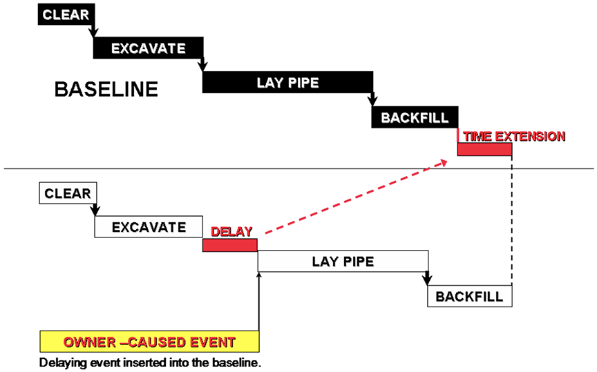
MIP 3.6 simulates an impact scenario by adding a new activity or relationship in an existing CPM network model. Activities and logic representing delays or changes are added into a CPM network model to determine their hypothetical impact on project milestones. “MIP 3.6 can be used prospectively or retrospectively.” [ 1, page 70 ]. Figure 5 illustrates the MIP 3.6 method (modeled, additive, single base analysis) applied to a delayed start of laying pipe.

Figure 5 
Modeled, Additive, Single Base Method
(Reprinted with permission of AACE® International) [ 1, page 70 ]

Limitations of MIP 3.6 include:

• It is a hypothetical model that does not account for changes in critical path and actual progress during construction (when applied to a baseline schedule).
• “Accuracy of the duration of critical path impact for any given delay event degrades in proportion to the chronological distance of the delay event from the data date.” [ 1, page 75 ].

3.7    MODELED / ADDITIVE / MULTIPLE BASE

MIP 3.7 “consists of the insertion or addition of activities representing delays or changes into a network analysis model representing a plan to determine the hypothetical impact of those inserted activities to the network.” [ 1, page 75 ]. While RP 29R‑03 states that “MIP3.7 is a retrospective analysis”, it is also commonly used prospectively as the project progresses. [ 1, page 76 ]. For example, see RP 29R‑03, Section 5.1, which states, “Some contracts … require that all requests for time extension (either during the life of the project or at the end of the job) be substantiated through the use of a prospective TIA (similar to MIP 3.7).” [ 1, page  126 ].

Limitations of MIP 3.7 are similar to MIP 3.6 except that compared to MIP 3.6, the periodic nature of MIP 3.7 incorporates as-built progress data and logic changes. MIP 3.7 is more labor intensive than the simpler MIP 3.6.

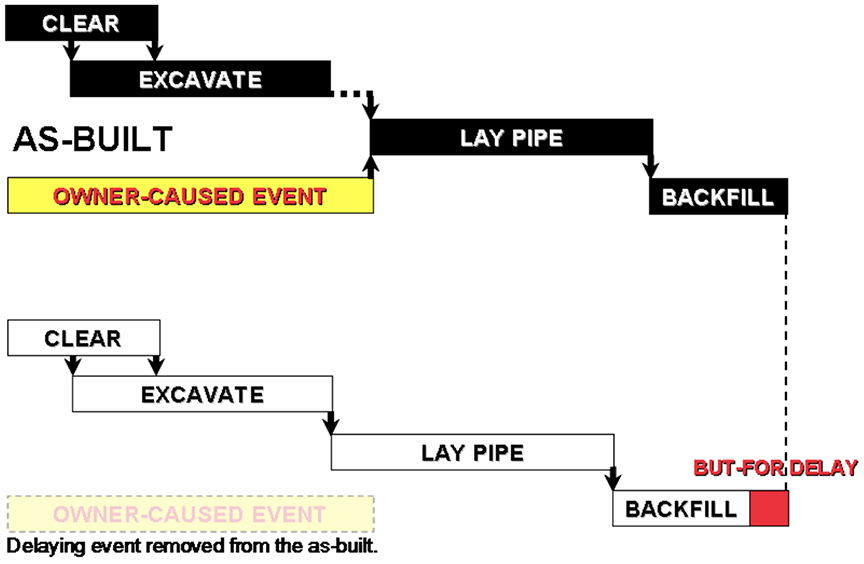
3.8    MODELED / SUBTRACTIVE / SINGLE SIMULATION

Both MIP 3.6 and 3.7 add activities or logic changes to a baseline or progress update schedules and compare the outcome to the as-built schedule (or next progress update). MIP 3.8 instead subtracts activities or changes from the as-built schedule. “The simulation consists of the extraction of entire activities or a portion of the as-built durations representing delays or changes from a network analysis model representing the as-built condition of the schedule to determine the impact of those extracted activities on the network.” [ 1, page 82 ]. “The subtractive simulation is performed on one network analysis model representing the as-built.” [ 1, page 82 ]. The outcome would be the actual progress of the project “but-for” the subtracted delays. The difference between the as-built schedule and the but-for schedule quantifies the incremental delay caused by the deleted activities. Figure 6 illustrates MIP 3.8 and shows that, but-for an owner caused delay to the start of pipe laying, backfilling would have completed earlier.

Figure 6 
Modeled, Subtractive, Single Simulation Method
(Reprinted with permission of AACE® International) [ 1, page 82 ]

Limitations of MIP 3.8 include:

• “Perceived to be purely an after-the-fact reconstruction of events that does not refer to schedule updates used during the project.” [ 1, page 89 ]
• “Reconstructing the as-built schedule is very fact and labor intensive.” [ 1, page 89 ]
• The as-built durations, changes in scope, changes in construction sequencing and methodologies may not have been adequately updated by the project planner.

3.9    MODELED / SUBTRACTIVE / MULTIPLE BASE

MIP 3.9 applies MIP 3.8 subtractive simulation to the as-built durations of multiple network analysis models typically representing updated schedules. “MIP 3.9 considers … logic changes and, therefore, is thought to be more attuned to the perceived critical path….” [ 1, page 90 ].

Limitations of MIP 3.9 include:

• As for MIP 3.8, MIP 3.9 depends on the quality and completeness of the schedule updates. Varied scope and changed sequencing (change in means/methodology) not reflected in the updated schedule may skew the analysis.
• “Reconstructing the as-built schedule is very fact and labor intensive.” [ 1, page 97 ].
• As with MIP 3.8, any changes to duration, scope and relationship to mimic as‑built conditions must be based on facts (documents), opinions of witnesses (superintendent, project manager) and the forensic planner’s experience with construction work sequences.

4.    FACTORS TO CONSIDER WHEN SELECTING THE MOST APPROPRIATE SCHEDULE ANALYSIS METHOD

RP 29R‑03 identifies technical, legal, and practical considerations for selecting the most appropriate schedule analysis method. “Some methods are better suited for certain purposes than others.” [ 1, page 127, Figure 17 ]. Other critical constraints include quality of project records, access to project personnel and time available.

A given protocol will typically be better suited to representing one party’s side of a dispute. As a result, opposing counsel may question the impartiality of the methodology. Because the choice of schedule analysis method may be challenged during or before trial, practitioners should know how best to select a particular delay evaluation method and how to document their choice in anticipation of a possible challenge.

4.1    TECHNICAL CONSIDERATIONS

“[T]he selection of the analytical method should be based primarily on technical considerations related to the purpose, the timing, availability of data, and the nature and complexity of the delay and scheduling information.” [ 1, page 125 ].

4.2    PURPOSE OF THE ANALYSIS

“Generally, the purpose of forensic schedule analysis is to quantify delay, determine causation, and assess responsibility and financial consequences for delay.” [ 1, page 127 ]. The forensic schedule analyst first assesses the events that occurred on the project, then considers “issues such as concurrent delay, pacing delay, delay mitigation, etc.” [ 1, page 127 ]. If concurrent delay is a significant issue in the delay analysis, then the forensic schedule analyst should choose a method that specifically provides for concurrent delay identification and analysis.

Figure 17 summarizes the suitability of the nine MIP’s for some typical forensic uses of CPM schedules.

Figure 17 
Some Methods Are Better Suited for Certain Purposes than Others
(Reprinted with permission of AACE® International) [ 1, page 127 ]

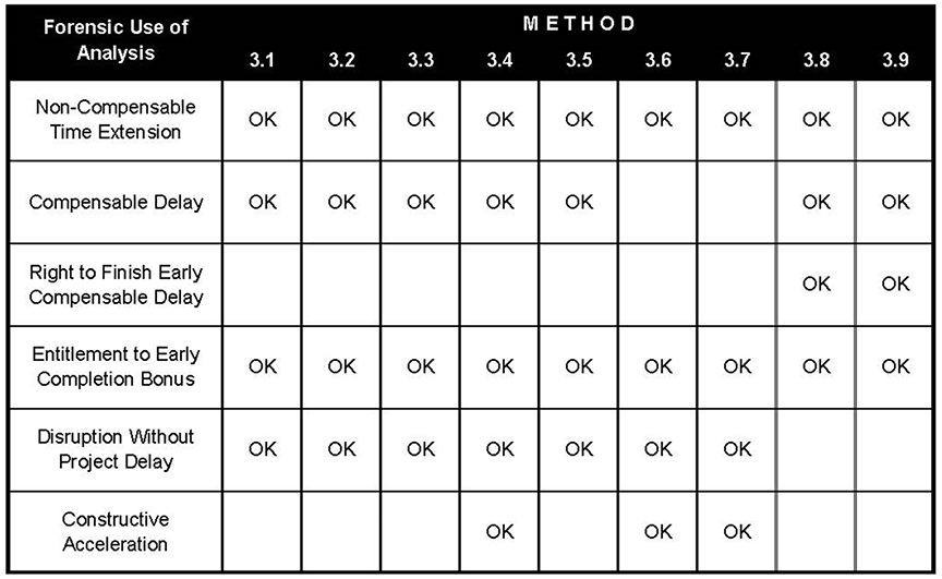
While, Figure 17 presents potential forensic uses of the nine schedule analysis methods, not all methods marked “OK” are commonly used for the purposes indicated. For example, MIP 3.8 and 3.9 are not typically used to demonstrate entitlement to a non-compensable time extension. An improvement to RP 29R‑03 would be to remove the “OK” marks on Figure 17 for “Non‑Compensable Time Extension” for MIP 3.8 and 3.9. Also, although not marked “OK”, MIP 3.6 and 3.7 can be used to demonstrate compensable delay as discussed in RP 29R‑03 Sections 3.6.I and 3.7.I. Another improvement to RP 29R‑03 would be to add the “OK” marks on Figure 17 for “Compensable Time Extension” for MIP 3.6 and 3.7. Finally, because MIPs 3.1 through 3.5 typically do not adequately consider concurrency and pacing issues, an improvement to RP 29R‑03 would be to remove the “OK” marks on Figure 17 for “Compensable Time Extension” for MIPs 3.1 through 3.5 because, in most US jurisdictions, if concurrent delays exist, typically neither party is entitled to compensable delay damages.

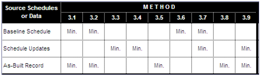
4.3    SOURCE DATA AVAILABILITY AND RELIABILITY

“[ T ]he choice of a particular forensic scheduling methodology is substantially influenced by the availability of source data that can be validated and determined reliable for the purpose of the analysis. If, for example, the project records show that there exists only a baseline schedule but no schedule updates for the duration of the project, then the observational MIP’s 3.3 and 3.4 cannot be utilized.” [ 1, page 128 ].

Only after reviewing the availability and reliability of the project documentation can the forensic scheduler formulate a plan and recommend a forensic schedule analysis method appropriate to the project and the analysis goals. Figure 18 presents “the source schedules that are required to implement the minimum basic protocol for each MIP.” [ 1, page 128 ].

Figure 18 
Source Data Validation Needed for Various Methods
(Reprinted with permission of AACE® International) [ 1, page 128 ]

4.4    COMPLEXITY OF THE DISPUTE

“When considering a forensic schedule analysis method, the forensic schedule analyst should do so with some knowledge of the complexity of the dispute in question and the number of events to be included in the forensic scheduling effort.” [ 1, page 128 ] “Some complex disputes can still be analyzed with a less complex analytical technique. And, some of the methods … may not require analysis of every activity on the schedule but can be focused on the critical path and sub-critical paths or on key events and activities only, to reduce both the cost and the complexity of the analysis.” [ 1, page 129 ].

4.5    LEGAL CONSIDERATIONS

“Having selected the technically appropriate analysis method based on these criteria, the analyst must now consider the legal criteria, which varies from one jurisdiction to another.” [ 1, page 125 ]. The schedule analyst should seek the advice of legal counsel “with specialized knowledge of the laws of the jurisdiction and forensic schedule analysis methods.” [ 1, page 125 ].

4.6    CONTRACTUAL REQUIREMENTS

“When a project is executed under a contract that specifies or mandates a specific schedule delay analysis method, then the choice of method is largely taken out of the hands of the forensic schedule analyst, and contract compliance is the prevailing factor. Some contracts, for example, now require that all requests for time extension (either during the life of the project or at the end of the job) be substantiated through the use of a prospective TIA (similar to MIP 3.7).” [ 1, page 126 ].

Given an unambiguous contract requirement describing the documentation or method to be used to support requests for time extensions or time related compensation, forensic schedule analysts should follow the contract requirements and the applicable codes and laws governing that contract. Unfortunately, as in the case of a contractual reference to a “but-for TIA”, not all contractual requirements that impact the forensic schedule analyst’s choice of methodology are clear and unambiguous.

4.7    FORUM FOR RESOLUTION AND AUDIENCE

The schedule analyst should consider “whether the claim is likely to settle in negotiation, mediation, arbitration (and if so, under what rules), or litigation (and if so, in which court). If there is good reason to believe that all issues are likely to be settled at the bargaining table, or in mediation, then the range of options for forensic scheduling methods is wide open as the audience is only the people on the other side and they may be motivated, persuaded or willing to make decisions based upon a forensic schedule analysis method different than that specified in the contract. Almost any option which is objective, accurately executed and is persuasive is legitimately open for consideration. On the other hand, if legal counsel believes that the issue will end up in court or a government agency board, then the range of options available may be considerably narrowed because many courts and boards have adopted their own rules concerning forensic scheduling.” [ 1, page 130 ].

4.8    LEGAL OR PROCEDURAL REQUIREMENTS

“Depending upon the forum for the dispute and the jurisdiction, the forensic schedule analyst must be aware of or ask about any contractual, legal, or procedural requirements that may impact the forensic analysis. There may be other contractual, legal, or procedural rules impacting forensic scheduling that the forensic scheduling analyst should consider when making a recommendation concerning which forensic scheduling methodology to use on a particular claim. Consultation with the client’s legal counsel on these issues is essential.” [ 1, page 130 ].

4.9    PRACTICAL CONSIDERATIONS

Legal and technical issues aside, other practical issues may also determine the choice of a particular forensic schedule analysis. “As in any commercial undertaking, while practical considerations are appropriate, these considerations must be secondary to the technical and legal considerations.” [ 1, pages 125-126 ].

4.10    SIZE OF THE DISPUTE

The size of the dispute and the amount in controversy typically plays a role in the choice of method. “In most situations, the choice of the forensic schedule analyst is constrained by how much a client has to spend to increase the probability of successful resolution of the dispute. This is most often determined by how much money is at stake. The forensic schedule analyst needs to recommend a forensic schedule analysis method that is both cost effective and suitable for the size of the dispute.” [ 1, page 128 ].

4.11    BUDGET FOR FORENSIC SCHEDULE ANALYSIS

Corresponding with the size and the complexity of the dispute is the client’s budget for the forensic schedule analysis. “If the client is prepared to spend only a small amount for a forensic schedule analysis effort, then the forensic schedule analyst should consider using less expensive forensic scheduling methods or cost saving alternatives – such as using the client’s in-house staff for certain tasks rather than outside consultant staff.” [ 1, page 129 ].

4.12    TIME ALLOWED FOR FORENSIC SCHEDULE ANALYSIS

For an analysis to be performed under time constraints, the forensic schedule analyst must consider “the time required for research, data validation, and claim team coordination which may be extensive, as well as production of the report.” [ 1, page 129 ].

The decision to perform a forensic schedule analysis is often not made early enough to allow complete flexibility in the choice of an analytical method, and the forensic schedule analyst may have a very limited timeframe in which to complete the work. If time constraints push the analyst to recommend short cuts or a method that can be completed in far less time than other forensic scheduling methods, then again the forensic schedule analyst should point out the risks of proceeding in this manner.

4.13    EXPERTISE OF THE FORENSIC SCHEDULE ANALYST AND RESOURCES AVAILABLE

If the forensic schedule analyst is experienced with only a few schedule analysis methods and may be challenged by the other side, “the forensic schedule analyst may be compelled to recommend use only of methods with which the analyst has experience. If the analyst determines that another method in which the analyst has little or no experience is more appropriate to the particular case then the analyst should be prepared to disclose that fact to the client. Additionally, if the forensic schedule analyst is to perform all analytical work individually with no assistance, the analyst may be constrained to recommend simpler methods which can be performed individually and will not require a staff of additional people processing data, making computer runs, etc.” [ 1, page 130 ].

4.14    CUSTOM AND USAGE OF METHODS ON THE PROJECT OR CASE

A final consideration is the past history of schedule analysis methods used during the project. “Typically, a forensic schedule analyst is not engaged until after preliminary negotiations have failed. Thus, the forensic schedule analyst needs to consider what delay analysis method was employed by the client and their staff earlier during the project, which was not acceptable to the other side in prior negotiations.” [ 1, page 130 ]. It is best to avoid a technique that has previously proven unsuccessful unless the scheduler can determine that the client staff performed the method erroneously in their early efforts, or that the basis for the previous rejection was clearly erroneous.

5.    CONCLUSION

All nine forensic schedule analysis methods have their appropriate uses, and their own strengths and limitations. All methods depend on the validation of source data. Considerable thought should be given to selecting the most appropriate methodology prior to starting a forensic schedule analysis, and this selection process must be accurately documented.

Not all of the eleven factors for consideration when selecting a forensic schedule analysis method will be applicable to all delay claims. Nevertheless, a prudent forensic schedule analyst should consider each of the above factors, as well as any other relevant factors that emerge, to determine which apply to the claim at hand. Once these factors are reviewed, including their potential synergistic effect upon each other, the forensic schedule analyst should discuss each applicable factor with the client and their legal counsel prior to recommending a particular method for the delay analysis. Special attention should be paid to the limits of an analyst’s own expertise. Insufficient attention to contractual limitations, forum of dispute, constraints on time and budget, or any of the other factors outlined above may lead to a poor choice of methodology that could cause substantial difficulties later on in claim settlement negotiations, arbitration, or litigation.

BIBLIOGRAPHY

No.      Description

  1        AACE® International Recommended Practice No. 29R-03, April 25, 2011 Revision, AACE International, Morgantown, WV

  2        Livengood, CFCC, PSP, John C.; Kelly, P.E., PSP, Patrick M., 2015, Forensic Schedule Analysis Methods: Reconciliation of Different Results, AACE International, Morgantown, WV

  3        D’Onofrio, P.E., Robert M., 2015, Ranking AACE International’s Forensic Schedule Analysis Methodologies, AACE International, Morgantown, WV

About the Author

Andrew Avalon, P.E., PSP, is Chairman of Long International, Inc. and has over 35 years of engineering, construction management, project management, and claims consulting experience. He is an expert in the preparation and evaluation of construction claims, insurance claims, schedule delay analysis, entitlement analysis, arbitration/litigation support and dispute resolution. He has prepared more than thirty CPM schedule delay analyses, written expert witness reports, and testified in deposition, mediation, and arbitration. In addition, Mr. Avalon has published numerous articles on the subjects of CPM schedule delay analysis and entitlement issues affecting construction claims and is a contributor to AACE® International’s Recommended Practice No. 29R‑03 for Forensic Schedule Analysis. Mr. Avalon has U.S. and international experience in petrochemical, oil refining, commercial, educational, medical, correctional facility, transportation, dam, wharf, wastewater treatment, and coal and nuclear power projects. Mr. Avalon earned both a B.S., Mechanical Engineering, and a B.A., English, from Stanford University.  Mr. Avalon is based in Orlando, Florida and can be contacted at aavalon@long-intl.com and (407) 445‑0825.

---

¹    “In legal disputes, [ professional judgment and knowledge of the subject matter ] is especially important where technical reasons for selection of a particular method must be reconciled with legal strategy,” Right On Schedule: Discussing Recommended Practice 29R‑03, Brian R. Dugdale, Watt Tieder (Fall 2011).

²    See http://www.cbca.gsa.gov/files/decisions/2015/LESTER_06-04-15_4659__YATES-DESBUILD_JOINT_VENTURE_V._DEPARTMENT_OF_STATE.pdf

Originally published by AACE International as CDR.2212 in the 2016 AACE International Transactions.
Reprinted with permission of AACE International, 1265 Suncrest Towne Centre Dr., Morgantown, WV 26505 U.S.A.
Telephone: +1 (304) 296-8444 | Facsimile: +1 (304) 291-5728 | web.aacei.org | Email: info@aacei.org
Copyright © 2016 by AACE International; all rights reserved.