1.    INTRODUCTION

The design phases of chemical processing plant and other industrial projects contain many potential risks. This is especially true when the project is for the first-of-a-kind deployment of new technology or when the performing organization has not previously successfully completed a similar project. These potential risks encompass several aspects of the project and final system, including: design phase project management issues such as cost overruns and schedule delays; procurement issues; constructability issues; operational and maintenance issues; and performance issues related to product quality, system capacity, and system availability.

This article describes three tools and methods that the author has found useful for identifying and mitigating risks during the design phases of chemical processing plant projects. Moreover, some of the risk mitigation methods described herein are generic in that they can also be applied to reduce risks associated with broader aspects of engineering and construction projects, such as project management risks and scheduling risks.

Section 2 of this article discusses the use of Failure Mode and Effects Analysis (FMEA) for the identification, prioritization, and mitigation of risks and includes an illustrative example. The use of the Kepner Tregoe (K-T) Analysis method for selecting the optimal solution for a given decision from several alternative solutions is discussed in detail, with an example, in Section 3. Finally, Section 4 discusses the importance of performing an availability analysis during the design phases of industrial processing plant projects. While Monte Carlo simulations are commonly used to identify and quantify cost and schedule risks, Long International discusses the use of Monte Carlo-based tools elsewhere¹ and further discussion is beyond the scope of this article.

2.    FAILURE MODE AND EFFECTS ANALYSIS

Failure Mode and Effects Analysis (FMEA) is a useful analysis tool for identifying, prioritizing, and mitigating risks. FMEA was developed by the U.S. military and is heavily used in the semiconductor industry.² This author has found FMEA to be a valuable tool for risk mitigation during the process design and development phases of chemical processing plant projects. FMEA can be especially useful for the first-of-a-kind deployment of new technologies or when the performing organization has not previously completed a similar project.

Performance of an FMEA is a team effort. Ideally, the FMEA team members should be of varied backgrounds and project roles to ensure the identification of risks from multiple points of view. FMEA participants can include contractor staff, such as project managers and key design engineers from various disciplines, as well as project owner staff, such as key maintenance and operations personnel. To facilitate the FMEA process, team members should be selected to fill the roles of FMEA leader (typically a senior engineer or project manager) and scribe (requires good spreadsheet and typing skills).

The FMEA process consists of two main tasks: the identification of risks and the subsequent prioritization and mitigation of risks, as discussed below in Sections 2.1 and 2.2, respectively. While commercial FMEA software is available and may generally improve the facilitation of the FMEA process, it is this author’s experience that a simple spreadsheet is generally sufficient.

The FMEA process is similar to, but different from, typical hazard and operability studies (HAZOPs). The primary difference is that HAZOPs focus on safety hazards, whereas the scope of an FMEA can cover safety as well as performance, quality, and reliability.³ Additionally, FMEA employs a bottom-up approach (as is discussed in Section 2.1 below) to ensure that all possible failure modes are captured, as opposed to the typical top-down approach of a HAZOP.⁴

2.1    FMEA: RISK IDENTIFICATION

The first step in the FMEA process is risk identification, which is typically accomplished through a team brainstorming exercise to identify all possible modes of failure and their associated effects. To aid in the subsequent prioritization and mitigation of the identified failure modes, it is important that the correct root cause and means of detection (e.g., process control system components) be determined for each of the identified failure modes.

The “what can go wrong” brainstorming exercise should generate an all-inclusive list of potential failure modes and risks. During the design phases of industrial processing plant projects, these risks may include but not be limited to:

• Potential safety issues during construction, operation, and maintenance of the system;
• Potential project management issues such as schedule delays and cost overruns associated with design complexity or the design of a first-of-a-kind system;
• Potential procurement issues such as availability of materials and long lead times, especially for first-of-a-kind systems that may require customized equipment fabrication or other hard-to-procure materials;
• Potential process or mechanical equipment issues that could impact equipment and/or system availability, including the lack of equipment redundancy;
• Potential process or mechanical equipment issues that could impact system capacity;
• Potential process or mechanical equipment issues that could impact product quality;
• Potential operational issues and concerns, including the potential for loss of utilities such as power, water, and compressed air;
• Potential maintenance access issues and concerns with respect to equipment layout, including means for moving equipment such as cranes, hoists, and fork lifts;
• Potential operations personnel access issues and concerns with respect to equipment layout, including sample port accessibility and means for refilling reagent supplies such as hoists and drum dollies;
• Potential for equipment damage during maintenance and/or operation; and
• Potential issues or concerns regarding the constructability of the as-designed system.

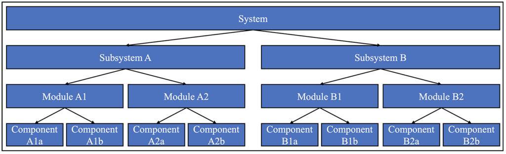
To ensure the identification of all possible failure modes, all modes of operation as well as the transitions between the various operating modes should be considered during the brainstorming exercise. It is also important to systematically work through all components and aspects of the system at hand in a logical manner such that no potential risks are overlooked. To achieve this, the FMEA brainstorming exercise should be a bottom-up analysis based either on the work breakdown structure (WBS) for the project or on a systems hierarchy such as that shown below in Figure 2‑1, where individual pieces of equipment are identified at the component level and are then integrated together at higher and higher levels of the system hierarchy.⁵ If the project was specified and/or designed based on systems engineering principles, the system hierarchy may be similar to the WBS for the project.

Figure 2‑1: Typical System Hierarchy

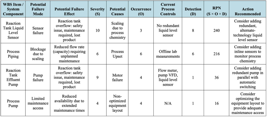
To facilitate the FMEA process, a template⁶ such as that shown below in Table 2‑1, which includes hypothetical entries for illustration purposes, should be used to capture the relevant information for each potential failure mode. The severity, occurrence, detectability, risk priority number (RPN), and action recommended columns are discussed in detail in Section 2.2 below.

Table 2‑1: Typical FMEA Template with Hypothetical Example Entries

2.2    FMEA: RISK RANKING AND MITIGATION

Once the failure modes and their effects have been identified as described above in Section 2.1, the next step in the FMEA process is to rank the relative risks of each line item so that the failure modes can be prioritized for mitigation in order from greatest to least risk. During this step of the FMEA, each of the identified risk items is scored using the following criteria:

• Severity (S): the severity of the failure mode effect, ranked on a scale of 1 (low risk) to 10 (high risk). Severity rankings of 1 typically indicate no noticeable effect on the process or product while severity rankings of 10 indicate a significant, potentially life threatening, safety issue.
• Occurrence (O): the frequency of occurrence of the failure mode, ranked on a scale of 1 (low risk) to 10 (high risk). Occurrence rankings of 1 indicate that failures are extremely rare while occurrence rankings of 10 indicate that failures are extremely frequent.
• Detection (D): the likelihood that the current process controls will detect the failure mode prior to its occurrence, ranked on a scale of 1 (low risk) to 10 (high risk).  Detection rankings of 1 indicate that current controls are almost certain to detect a failure prior to its occurrence while detection rankings of 10 indicate there is currently no detection for the failure mode.

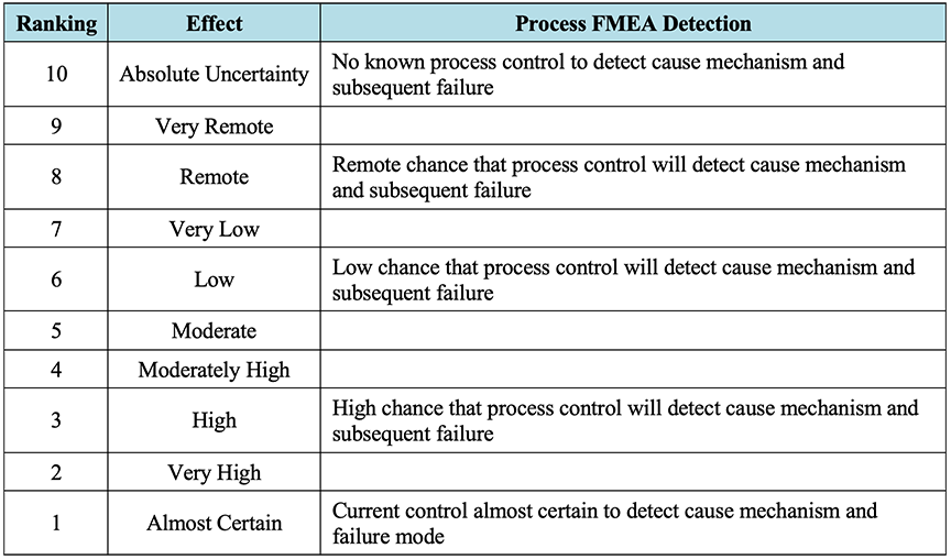
For reference, Table 2‑2, Table 2‑3,⁷ and Table 2‑4 below, adapted from “FMEA – Lean Manufacturing and Six Sigma Definitions,”⁸ depict typical example process FMEA ranking descriptions for severity, occurrence, and detection, respectively. It should be noted that the rankings are somewhat subjective, are provided herein as a general guide, and may need to be tailored to the FMEA at hand.⁹ Rankings should be finalized and agreed upon by members of the FMEA team prior to starting the scoring process.

Table 2‑2: Typical FMEA Severity Rankings

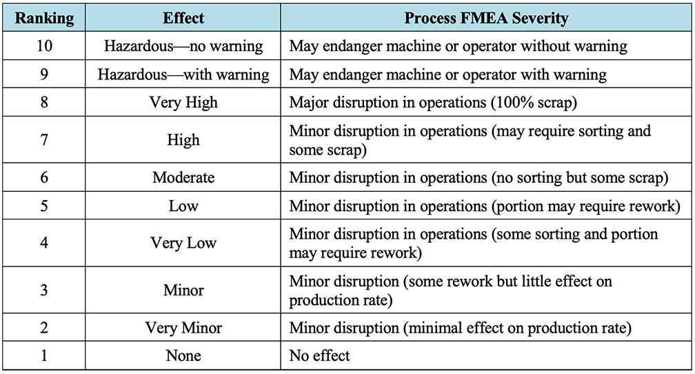
Table 2‑3: Typical FMEA Occurrence Rankings

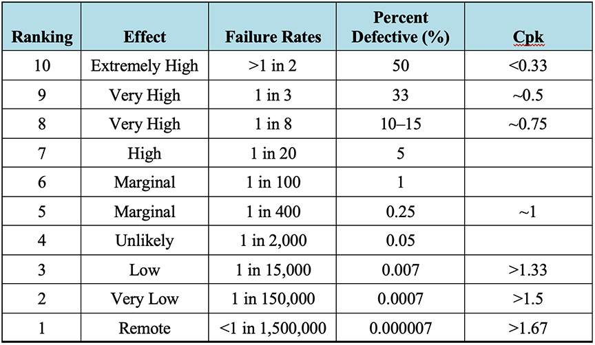
Table 2‑4: Typical FMEA Detection Rankings

Similar to the brainstorming of failure modes discussed in Section 2.1, the scoring of the identified failure modes should be performed as a team exercise because the quality of the resulting risk prioritization will benefit from the varied backgrounds and points of view of the various FMEA team members. Note that the scoring is somewhat subjective, rather than quantitative, and may be an iterative process. That is, once the FMEA team has scored all the failure modes, it is typically beneficial to review the assigned scorings and verify that the rankings of items scored earlier in the FMEA process are consistent with those scored later in the process, and that the scoring of failure modes with similar effects are consistent with each other.

Once the FMEA line items have been scored for severity, occurrence, and detection, the risk priority number (RPN) for each line item is calculated as the product of the three scores (i.e., RPN = S × O × D) as shown above in Table 2‑1. The higher the RPN, the greater the risk associated with a particular FMEA line item. Once the RPNs have been calculated, the FMEA template can be sorted in order of decreasing RPN to identify the highest risk line items.

In addition to scoring the FMEA line items for severity, occurrence, and detection, the FMEA team should brainstorm and record recommended actions for the mitigation of each risk as shown above in Table 2‑1. It is usually beneficial to re-score the FMEA line items with the assumption that the recommended actions have been completed and to compare the updated RPNs with the initial RPNs to show the resulting decrease in risk associated with each of the recommended actions. If the FMEA line items are re-scored, it is recommended that additional columns be added to the FMEA template to record these additional scores, such that the original scores are preserved in the record.

Once the identified risks have been sorted by RPN, the FMEA team (or project management, as appropriate) can weigh the risks associated with each failure mode against the effort, cost, and project budget associated with each of the proposed mitigations to determine which of the recommended actions will be implemented. One industry expert cites a rule of thumb that any risk with an RPN greater than 80 should be addressed.¹⁰ Typically, all potential safety issues and other critical issues with high severity scorings should be addressed, although this may not be necessary if the probability of occurrence is close to zero or if robust detection capabilities exist. Finally, the FMEA team should consider implementing any identified low-cost mitigations such as those that only require straightforward control system programming updates or minor changes to operational or maintenance procedures.

3.    KEPNER TREGOE (K-T) DECISION ANALYSIS

Kepner and Tregoe describe a well-known decision analysis tool, commonly known as a K-T Analysis, for selecting the best option from several alternative solutions for a given decision.¹¹ This author has found the K-T Analysis to be a valuable tool for reducing risk when analyzing design trade-offs and procurement bids during the process design and procurement phases of chemical processing plant projects. Additionally, a K-T Analysis can provide traceability and transparency for critical design and procurement decisions. The K-T Analysis can be performed either as a team exercise or by a qualified individual, with subsequent review by a subject matter expert and/or project manager, as applicable.

The first step of the K-T Analysis is to define the decision process, which consists of clearly stating the decision at hand, determining the objectives of the decision (both “must-haves” and “wants”), and subjectively weighting the “wants” on a scale of 1 (least important) to 10 (most important). Once the K-T Analysis has been defined, the various alternative solutions for the decision at hand can be analyzed. The analysis consists of screening each of the alternative solutions against the “must-have” criteria, scoring the “wants” for any alternative solutions that satisfied the “must-have” criteria, and calculating the weighted scores for the “wants” for each of the alternative solutions. The alternative with the highest weighted score is then selected as the tentative choice, with the finalization of the choice pending an analysis of the associated risks. The K-T Analysis method is best illustrated by example.

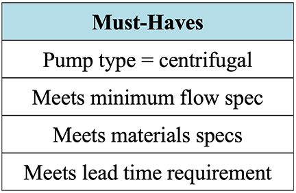
In the following simplified, hypothetical example, a K-T Analysis is used to select the best option from four bids received in response to a Request for Quote (RFQ) for a centrifugal pump. The “must-have” criteria were determined to include verification that the vendor bids met the requested pump type (centrifugal), met the minimum flow specification, were of the material of construction specified in the RFQ, and met the lead time requirement as shown below in Table 3‑1. Generally, when using a K-T Analysis to analyze procurement bids, the “must-have” criteria should encompass all hard requirements stated in the RFQ.

Table 3‑1: K-T Analysis Example: “Must-Have” Criteria

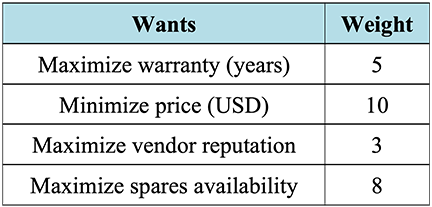
In this example, the “want” criteria were determined to be: maximize the warranty period; minimize the price; maximize vendor reputation; and maximize spares availability. Generally, when using a K-T analysis to analyze procurement bids, the “want” criteria can encompass all desirable qualities of the equipment to be purchased including minimizing both capital and operational costs while maximizing quality and performance.

The relative weights, based on a scale of 1 (least important) to 10 (most important), were assigned as shown below in Table 3‑2 such that a weight of 10 was assigned to the criterion deemed most important (price) and the remaining criteria were weighted relative to the importance of the price criterion. For example, a weight of 5 indicates that particular criterion was deemed to be half as important as the price criterion. While the weights are subjective and chosen at the discretion of the analyst (or analysis team), it is important to finalize the weights prior to scoring the various alternative solutions to prevent the introduction of bias into the analysis.

Table 3‑2: K-T Analysis Example: “Want” Criteria and Weights

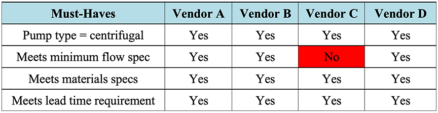
Once the criteria and weights have been determined, the next step is to screen each of the four bids against the “must-have” criteria. As shown in Table 3‑3 below, the analysis of the four hypothetical bids showed that all the “must-have” criteria were satisfied except for the flow specification for the bid received from Vendor C. Because Vendor C failed to meet the “must-have” criteria, its bid was eliminated from consideration.

Table 3‑3: K-T Analysis Example: “Must-Have” Screening

The next step is to score each of the remaining three bids against the “want” criteria on a scale of 1 (least favorable) to 10 (most favorable). Note that the “want” criteria consist of two types of criteria: those that need to be scored subjectively (vendor reputation and spares availability) and those that can be scored quantitatively (warranty period and price). Although the scores for the warranty period and price can also be set subjectively based on their relative values for each of the three bids, this author recommends that the scores should be determined quantitatively.

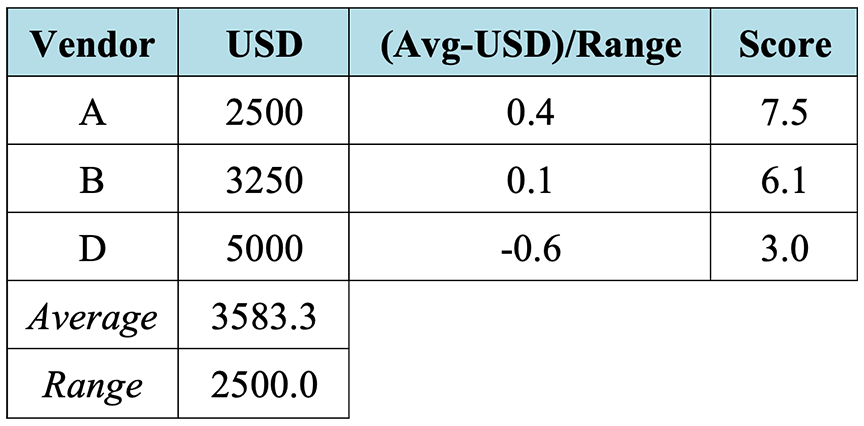
To determine the scores for the warranty period and price quantitatively, the warranty period and price specified in each of the three bids should first be normalized to a scale of 1 (least favorable) to 10 (most favorable). One way to normalize the data is to normalize with respect to the average¹² as shown below in Table 3‑4 and Table 3‑5 for the warranty period and price data, respectively.¹³ Once the data has been normalized, the data can be re-scaled from the range of the normalized data (assumed to be -1 to 1) to the desired scoring scale of 1 to 10. This is accomplished by multiplying the normalized data by 4.5 and adding 5.5.¹⁴

Table 3‑4: K-T Analysis Example: Warranty Period Data Normalization

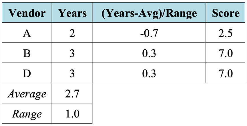
Table 3‑5: K-T Analysis Example: Price Data Normalization

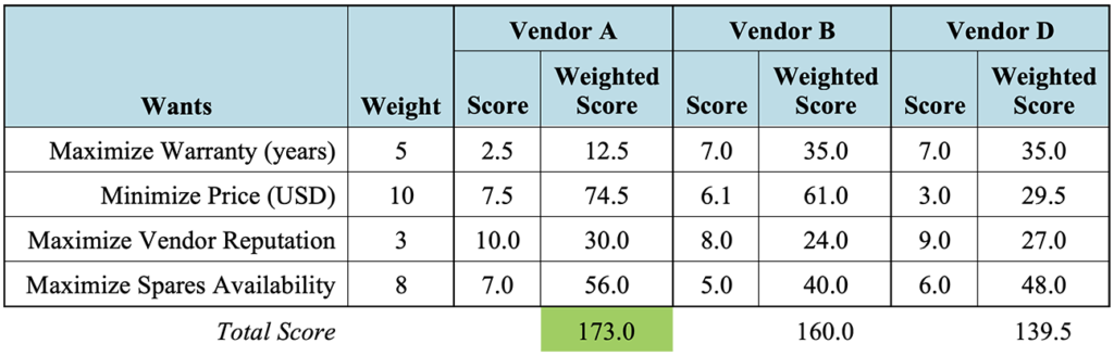
With the quantitative scores for the warranty period and price determined, the subjective scores for the vendor reputation and spares availability can be assigned and the weighted scores calculated as shown below in Table 3‑6. In this example, Vendor A received the highest total score, indicating that its bid is the tentative choice.

Table 3‑6: K-T Analysis Example: “Want” Scoring

The final step of the K-T Analysis is to analyze the risks associated with the tentative choice. Kepner and Tregoe discuss identifying and then rating risks on the basis of probability and seriousness, similar to the occurrence and severity FMEA categories discussed above in Section 2.2.¹⁵ They stress that this final risk analysis is not a comparison of risks among the alternative solutions, but that each alternative should be examined separately.¹⁶ Once the risks have been analyzed for the tentative choice, if it is determined that there are no significant risks that cannot be mitigated, the tentative choice can be finalized as the best balanced choice.

4.    AVAILABILITY ANALYSIS AND EQUIPMENT REDUNDANCY

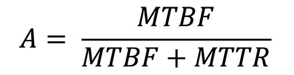
Availability is defined as the percentage of time that a piece of equipment (component), module, subsystem, or the entire system¹⁷ is operational, and it is driven by time loss,¹⁸ as shown below in Equation 4‑1,¹⁹ where A is availability. Reliability is the probability that a component, module, subsystem, or entire system will meet performance requirements for a desired time duration and is usually measured as mean time between failures (MTBF) or mean time to repair (MTTR).²⁰ Reliability can be considered a subset of availability,²¹ with an alternate calculation of availability being dependent on these reliability metrics as is shown below in Equation 4‑2.²²

Equation 4‑1: Availability as a Function of Time

Equation 4‑2: Availability as a Function of Reliability Metrics

For projects such as the design and construction of chemical processing facilities or other industrial plants, a system availability requirement, which will typically be demonstrated and verified during performance testing, is usually specified in the contract documents. System-level availability is dependent on the availability of each of the individual components that comprise the system, as is shown below in Equation 4‑3 for system components arranged in series and Equation 4‑4 for system components arranged in parallel.²³ Therefore, individual pieces of equipment with relatively low availability pose a risk because they can significantly impact the availability of the entire system.

Equation 4‑3: Availability of n Components in Series

Equation 4‑4: Availability of n Redundant Components in Parallel

In some cases, system availability can be significantly increased during the design phases by improving the availability of individual system components that exhibit inherently low availability. One way to accomplish this is by adding redundant, parallel equipment to the design such that if the main equipment fails, the backup unit is available to support continued operations. There are obviously trade-offs between the added costs and space requirements of additional equipment and the resulting increase in availability, such that including redundancy for all equipment is unlikely to be feasible. However, system availability can sometimes be significantly increased by including redundancy for smaller pieces of equipment such as smaller processing pumps that are prone to failure or specific sections of piping that are prone to corrosion or scaling.

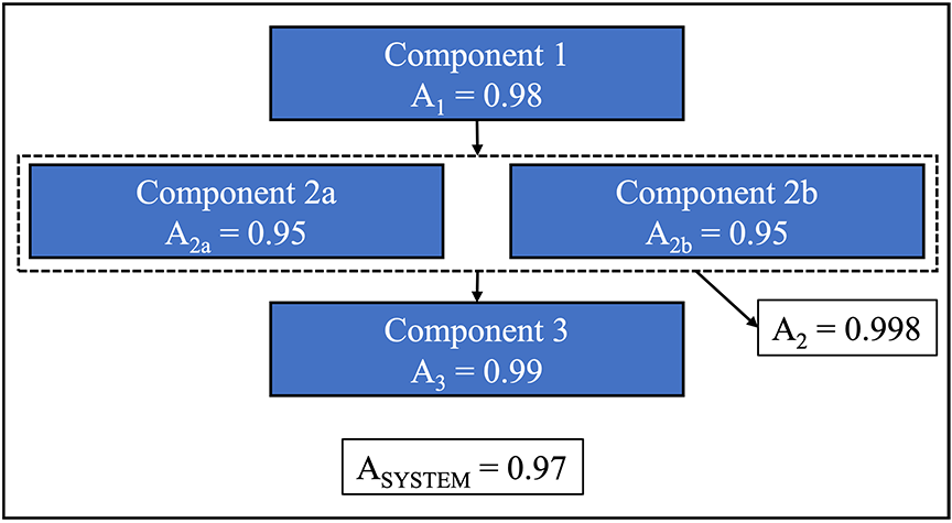
To illustrate this point, consider the example shown in the figures below. Figure 4‑1 depicts a system comprised of three components, where the system-level availability is significantly impacted by the relatively low availability of Component 2. Figure 4‑2 shows that the addition of redundant parallel equipment for Component 2 results in a significant increase in the overall availability of the system.

Figure 4‑1: Example System Availability for Three Components in Series

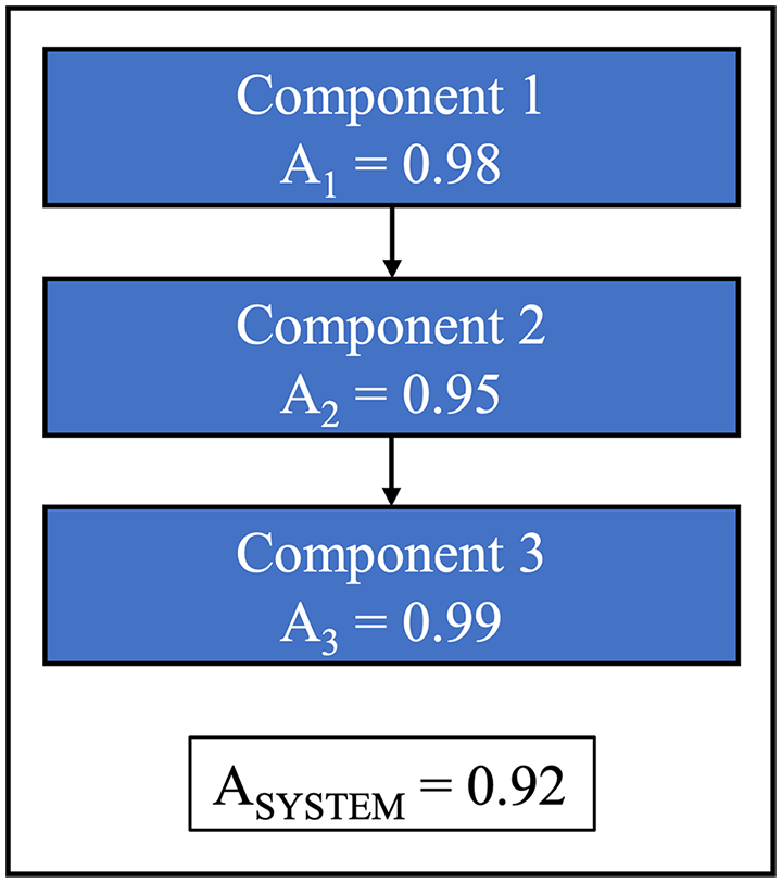
Figure 4‑2: Example System Availability with Added Parallel Redundancy

This author has found system availability analysis to be a useful tool for reducing system design risk through the prediction of system availability and comparison to the availability requirement, the identification of the availability-limiting equipment, and the determination of the benefit of adding redundant equipment in parallel. Availability analysis can be especially useful for the first-of-a-kind deployment of new technologies or when the performing organization has not previously completed a similar project.

For systems where the process flow diagram (PFD) is relatively simple and the availabilities of the individual components are known either from vendor data or previous experience with similar equipment, the availability analysis may be able to be accomplished manually using Equation 4‑3 and Equation 4‑4 above. For more complicated systems, or in cases where equipment availability or reliability are not well known, it may be beneficial for the design engineer to utilize commercially available software packages, which typically contain reliability data or distributions for various pieces of industrial equipment and are capable of simulating system-wide availability based on user-entered system block diagrams. Further discussion or review of these commercially available software packages is beyond the scope of this article.

About the Author

Eric J. Klein, Ph.D., P.E., PMP, is a Vice President of Long International. He has over 20 years of industrial experience as a Technical Leader, Project Manager, and Consultant in engineering, procurement, and construction (EPC), manufacturing, and research and development (R&D) environments. Dr. Klein is skilled in corporate leadership and has significant experience leading cross-functional teams to design, build, commission, start up, and test chemical processing systems in the power generation and semiconductor manufacturing industries. He possesses project management experience for multimillion-dollar capital projects including earned value management, risk management, contract and scope of work negotiation, technical project proposals, cost estimating, change control, requests for information (RFI), change order management, design management, and equipment procurement oversight. Prior to joining Long International, Dr. Klein held the positions of Chief Technology Officer, Vice President of Chemical Systems, Director of Chemical and Process Engineering, Staff Technologist, and Senior Process Engineer. Dr. Klein is based in the Denver, Colorado area and can be contacted at eklein@long-intl.com and (720) 982-3813.

---

¹   See Hulett, David T. and Avalon, Andrew. “Integrated Cost and Schedule Risk Analysis,” Long International, and Carter, Rod C. and Long, Richard J. “Applications of Monte Carlo Simulations in Dispute Resolution and Claims Work,” Long International.

²   “Failure Mode and Effects Analysis” (18 August 2022), Wikipedia. See https://en.wikipedia.org/wiki/Failure_mode_and_effects_analysis.

³   Carlson, Carl (2016), “FMEA Corner: Hazard Analysis,” in Reliability HotWire. See https://www.weibull.com/hotwire/issue189/fmeacorner189.htm.

⁴   Marion (2017), “What is FMEA and How is it Different from Hazard Analysis?,” in SoftComply Blog. See https://softcomply.com/what-is-fmea-and-how-is-it-different-from-hazard-analysis/.

⁵   When employing the system hierarchy approach, it is recommended that clear delineations between the various components, modules, and subsystems be shown on the process flow diagrams (PFDs) and/or piping and instrumentation diagrams (P&IDs) to assist in the brainstorming process.

⁶   Forrest, George (2013). “FMEA (Failure Mode and Effects Analysis) Quick Guide,” ISIXSIGMA. See https://www.isixsigma.com/tools-templates/fmea/fmea-quick-guide/.

⁷   “Cpk,” shown in Table 2‑3 below, is a measure of process capability, the details of which are beyond the scope of this article.

⁸   FMEA – Lean Manufacturing and Six Sigma Definitions. See https://www.leansixsigmadefinition.com/glossary/fmea/.

⁹   For example, in the case of an FMEA for a continuous industrial processing plant, it may be desirable to revise the severity and occurrence descriptions to include decreases in capacity, availability, or product quality. It may also be necessary to revise the ratings descriptions in the case of non-process-related risks such as those related to project management or procurement issues.

¹⁰   Ghosh, Mayukh (2010).  “A Guide to Process Failure Mode Effects Analysis (PFMEA),” PEX Network. See https://www.processexcellencenetwork.com/lean-six-sigma-business-performance/articles/process-failure-mode-effects-analysis-pfmea.

¹¹   Kepner, Charles and Tregoe, Benjamin (1981). The New Rational Manager: An Updated Edition for a New World, Princeton Research Press, pp. 107–182.

¹²   Narasimhan, K. Adith (2021). “Mean Normalization and Feature Scaling—A Simple Explanation,” Analytics Vidhya. See https://medium.com/analytics-vidhya/mean-normalization-and-feature-scaling-a-simple-explanation-3b9be7bfd3e8.

¹³   Note that in the case of the warranty period, the average is subtracted from the data, while in the case of the price, the data is subtracted from the average. This is because the “want” criteria are to maximize the warranty period and minimize the price.

¹⁴   These figures were determined assuming a straight-line mapping, where y = mx + b, of normalized data on a scale of -1 to 1 to scaled data on a scale of 1 to 10.

¹⁵   Kepner, Charles and Tregoe, Benjamin (1981). The New Rational Manager: An Updated Edition for a New World, Princeton Research Press, pp. 127–134.

¹⁶   Id., p. 132.

¹⁷   See Figure 2‑1 above for depiction of system hierarchy.

¹⁸   Raza, Muhammad (2020). “Reliability vs. Availability: What’s the Difference,” DevOps Blog. See https://www.bmc.com/blogs/reliability-vs-availability/.

¹⁹   Note that the down time in Equation 4‑1 includes both scheduled and unscheduled downtime.

²⁰   Raza, Muhammad (2020). “Reliability vs. Availability: What’s the Difference,” DevOps Blog. See https://www.bmc.com/blogs/reliability-vs-availability/.

²¹   Ibid.

²²   “System Reliability and Availability,” EventHelix Blog. See https://www.eventhelix.com/fault-handling/system-reliability-availability/.

²³   Ibid.

Copyright © Long International, Inc.